Time-varying hazard ratio plot
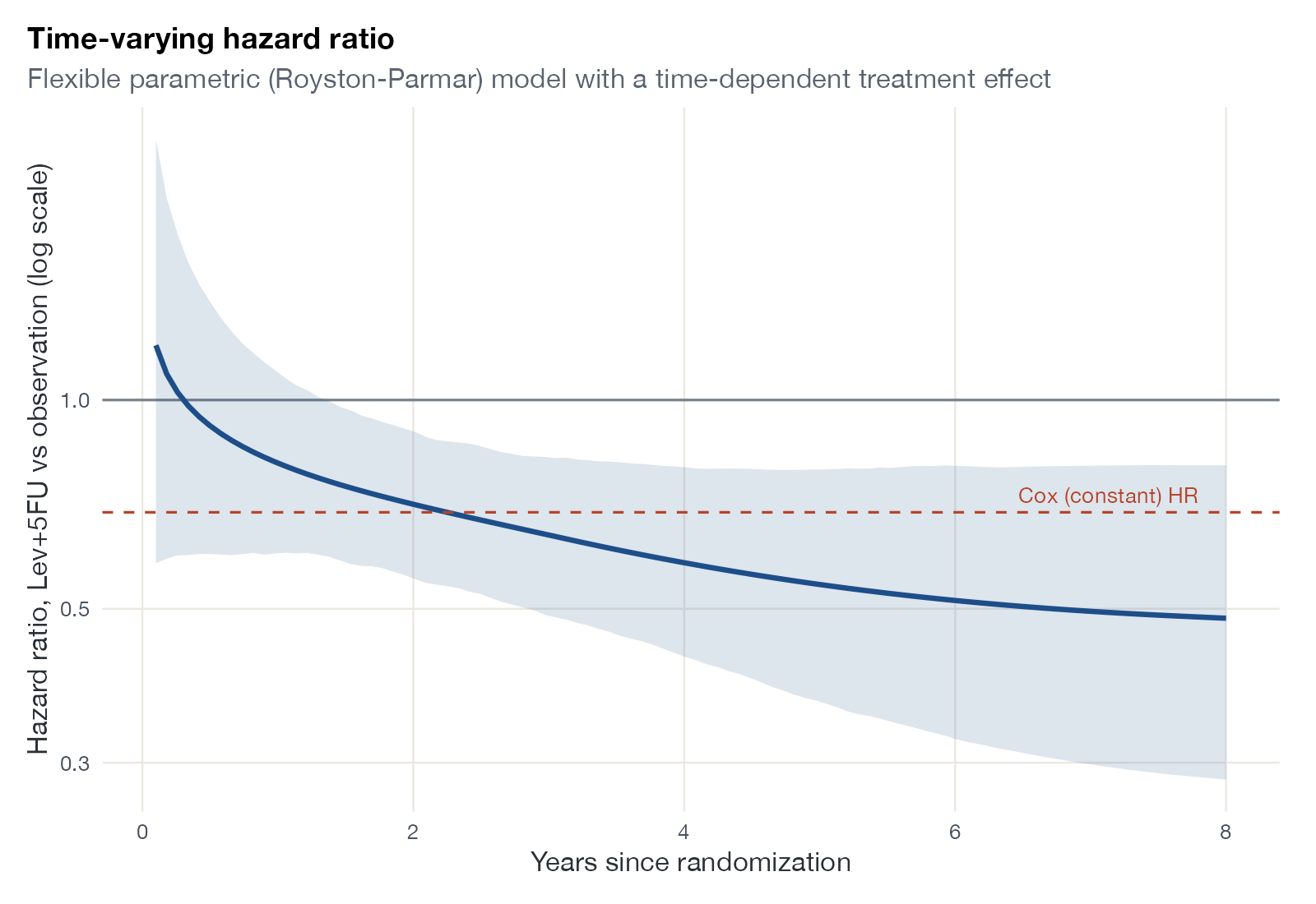
Hazard ratio over time, fractional polynomial or spline hazard ratio curve
survival::colon.
flexsurv::hr_flexsurvreg() (shown), multinma M-spline models, fractional polynomial NMA code; Stata stpm2
What it shows
When hazards are not proportional, the treatment effect is a curve, not a number. Flexible parametric (Royston-Parmar) models, fractional polynomial NMA (Jansen; Ouwens and colleagues), and M-spline models in multinma all estimate the hazard ratio as a function of time. Plotting that function, ideally for each comparison in a network, shows when a treatment helps, when its effect wanes, and how misleading a single average hazard ratio can be.
How to read it
- Horizontal axis: time since randomization.
- Vertical axis: hazard ratio on a log scale.
- Curve and band: time-varying hazard ratio and its 95% CI.
- Dashed line: the constant hazard ratio from a proportional hazards model.
Interpretation
The benefit of levamisole plus 5-FU is small in the first months, the hazard ratio is near 1 at the start and falls steadily to about 0.5 by year 8. The Cox model’s single hazard ratio of 0.69 averages over this pattern. In this trial the formal Schoenfeld test is not significant ( = 0.28$), and the confidence band is wide early, so the time trend is suggestive rather than established.
Pitfalls
- Hazard ratios over time are hard to interpret causally because of selection among survivors; pair them with survival or RMST differences.
- Estimates at late times rest on few patients; the band widens accordingly.
- Flexible models can overfit; compare with simpler models using information criteria.
Code
library(survival)
library(flexsurv)
library(ggplot2)

# Colon cancer adjuvant trial: death, observation vs levamisole + 5-FU
data(colon, package = "survival")
d <- subset(colon, etype == 2 & rx %in% c("Obs", "Lev+5FU"))
d$rx <- droplevels(d$rx)
d$years <- d$time / 365.25

# Royston-Parmar spline model with a time-varying treatment effect
fit <- flexsurvspline(Surv(years, status) ~ rx + gamma1(rx), data = d, k = 2)
hr <- hr_flexsurvreg(fit, t = seq(0.1, 8, length.out = 100),
                     newdata = data.frame(rx = c("Obs", "Lev+5FU")))

ggplot(hr, aes(t, est)) +
  geom_hline(yintercept = 1, colour = "#7a828c") +
  geom_ribbon(aes(ymin = lcl, ymax = ucl), fill = "#1d4e89", alpha = 0.15) +
  geom_line(colour = "#1d4e89", linewidth = 1.1) +
  geom_hline(yintercept = exp(coef(coxph(Surv(years, status) ~ rx, data = d))),
             linetype = "dashed", colour = "#b5452b") +
  annotate("text", x = 7.8, y = exp(coef(coxph(Surv(years, status) ~ rx, data = d))),
           label = "Cox (constant) HR", vjust = -0.6, hjust = 1, colour = "#b5452b", size = 3.4) +
  scale_y_log10() +
  labs(x = "Years since randomization", y = "Hazard ratio, Lev+5FU vs observation (log scale)",
       title = "Time-varying hazard ratio",
       subtitle = "Flexible parametric (Royston-Parmar) model with a time-dependent treatment effect")
References
- Royston P, Parmar MKB. Flexible parametric proportional-hazards and proportional-odds models for censored survival data, with application to prognostic modelling and estimation of treatment effects. Stat Med. 2002;21:2175-2197. doi:10.1002/sim.1203
- Jansen JP. Network meta-analysis of survival data with fractional polynomials. BMC Med Res Methodol. 2011;11:61. doi:10.1186/1471-2288-11-61