Bayesian node-split density plot
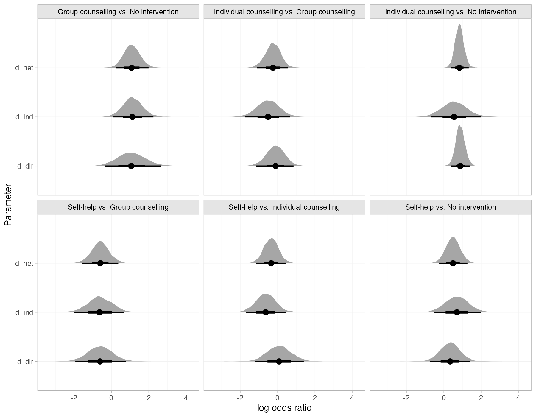
Posterior densities of direct, indirect, and network estimates
multinma::smoking.
multinma::nma(consistency = "nodesplit") + plot(), gemtc::mtc.nodesplit()
What it shows
The Bayesian version of the node-splitting forest plot. A separate model is fitted for each comparison with both direct and indirect evidence, splitting the parameter for that comparison into a direct and an indirect part. Plotting the three posteriors (direct, indirect, and the consistency model’s network estimate) shows not just whether intervals overlap but how the distributions differ in location and spread.
How to read it
- Panels: split comparisons.
- Rows: direct (
d_dir), indirect (d_ind), and network (d_net) estimates. - Densities and intervals: posterior density, median, and 66% and 95% credible intervals.
- Agreement: direct and indirect densities that overlap heavily.
Interpretation
Direct and indirect posteriors overlap for every comparison. The largest shift is for self-help versus individual counseling (direct near 0.1, indirect near −0.6 on the log odds scale), but the posteriors are wide and overlap substantially. Combined with the dev-dev plot, there is no evidence of inconsistency in this network.
Pitfalls
- Each split requires its own model; with large networks this is computationally heavy.
- Overlapping densities do not prove consistency when both are wide.
- In random-effects models, heterogeneity is re-estimated in each split model and can absorb inconsistency.
Code
library(multinma)

net <- set_agd_arm(smoking, study = studyn, trt = trtc, r = r, n = n,
                   trt_ref = "No intervention")

# Fit one node-splitting model per comparison with both direct and indirect evidence
fit_ns <- nma(net, trt_effects = "random", consistency = "nodesplit",
              prior_intercept = normal(scale = 100), prior_trt = normal(scale = 100),
              prior_het = half_normal(scale = 5), seed = 2026)

# Posterior densities of the direct, indirect, and network estimates per comparison
plot(fit_ns, stat = "halfeye") +
  ggplot2::labs(x = "log odds ratio")
References
- Dias S, Welton NJ, Caldwell DM, Ades AE. Checking consistency in mixed treatment comparison meta-analysis. Stat Med. 2010;29:932-944. doi:10.1002/sim.3767
- van Valkenhoef G, Dias S, Ades AE, Welton NJ. Automated generation of node-splitting models for assessment of inconsistency in network meta-analysis. Res Synth Methods. 2016;7:80-93. doi:10.1002/jrsm.1167