Meta-regression bubble plot
Bubble plot, meta-regression scatter plot
metadat::dat.bcg.
metafor::regplot(), orchaRd::bubble_plot(); Stata estat bubbleplot
What it shows
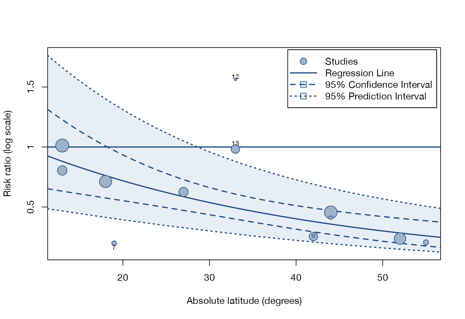
The bubble plot is the graphical form of meta-regression. Each study is a bubble at its moderator value and its effect estimate, sized by the weight it receives. The fitted meta-regression line, with confidence and prediction bands, shows the estimated relationship between the moderator and the effect. It is the main exploratory tool for heterogeneity and a natural precursor to asking whether population adjustment is needed.
How to read it
- Horizontal axis: the study-level moderator.
- Vertical axis: the effect estimate (log scale for ratios).
- Bubble area: weight in the meta-regression, usually inverse of \(v_i + \hat\tau^2\).
- Solid line: fitted relationship; dashed: 95% confidence band; dotted: 95% prediction band.
- Reference line: no effect.
Interpretation
The risk ratio falls with distance from the equator: the log risk ratio decreases by 0.029 per degree (95% CI −0.043 to −0.015), so every 10 degrees multiplies the risk ratio by about 0.75. Latitude accounts for about 76% of the between-study variance (\(\tau^2\) drops from 0.31 to 0.08), though residual heterogeneity remains.
Pitfalls
- Associations across studies are observational and prone to ecological bias. A relation between a study’s mean age and its effect is not evidence that the effect varies with age within patients.
- Meta-regression needs enough studies (a rough rule is ten per covariate) and enough spread in the moderator.
- Extrapolating the line beyond the observed range of the moderator is unsupported.
- Testing many moderators produces false positives; pre-specify them.
Code
library(metafor)

data(dat.bcg, package = "metadat")
dat <- escalc(measure = "RR", ai = tpos, bi = tneg, ci = cpos, di = cneg,
              data = dat.bcg)

# Random-effects meta-regression on absolute latitude of the trial site
fit <- rma(yi, vi, mods = ~ ablat, data = dat, method = "REML")

regplot(
  fit,
  mod = "ablat",
  xlab = "Absolute latitude (degrees)",
  ylab = "Risk ratio (log scale)",
  transf = exp, refline = 1,
  bg = "#9fb3c8", col = "#1d4e89",
  shade = "#e8eef6", lcol = "#1d4e89", lwd = 2,
  pi = TRUE, legend = TRUE, label = "piout", labsize = 0.7
)
meta esize tpos tneg cpos cneg, esize(lnrratio) random(reml)
meta regress ablat
estat bubbleplotReferences
- Thompson SG, Higgins JPT. How should meta-regression analyses be undertaken and interpreted? Stat Med. 2002;21:1559-1573. doi:10.1002/sim.1187
- Colditz GA, Brewer TF, Berkey CS, et al. Efficacy of BCG vaccine in the prevention of tuberculosis: meta-analysis of the published literature. JAMA. 1994;271:698-702. doi:10.1001/jama.1994.03510330076038
- Viechtbauer W. Conducting meta-analyses in R with the metafor package. J Stat Softw. 2010;36(3):1-48. doi:10.18637/jss.v036.i03