Treatment effect response surface
Interaction surface, two-modifier contour plot
STC
ML-NMR
ML-UMR
The conditional treatment effect over a grid of two effect modifiers, with the observed data support overlaid.
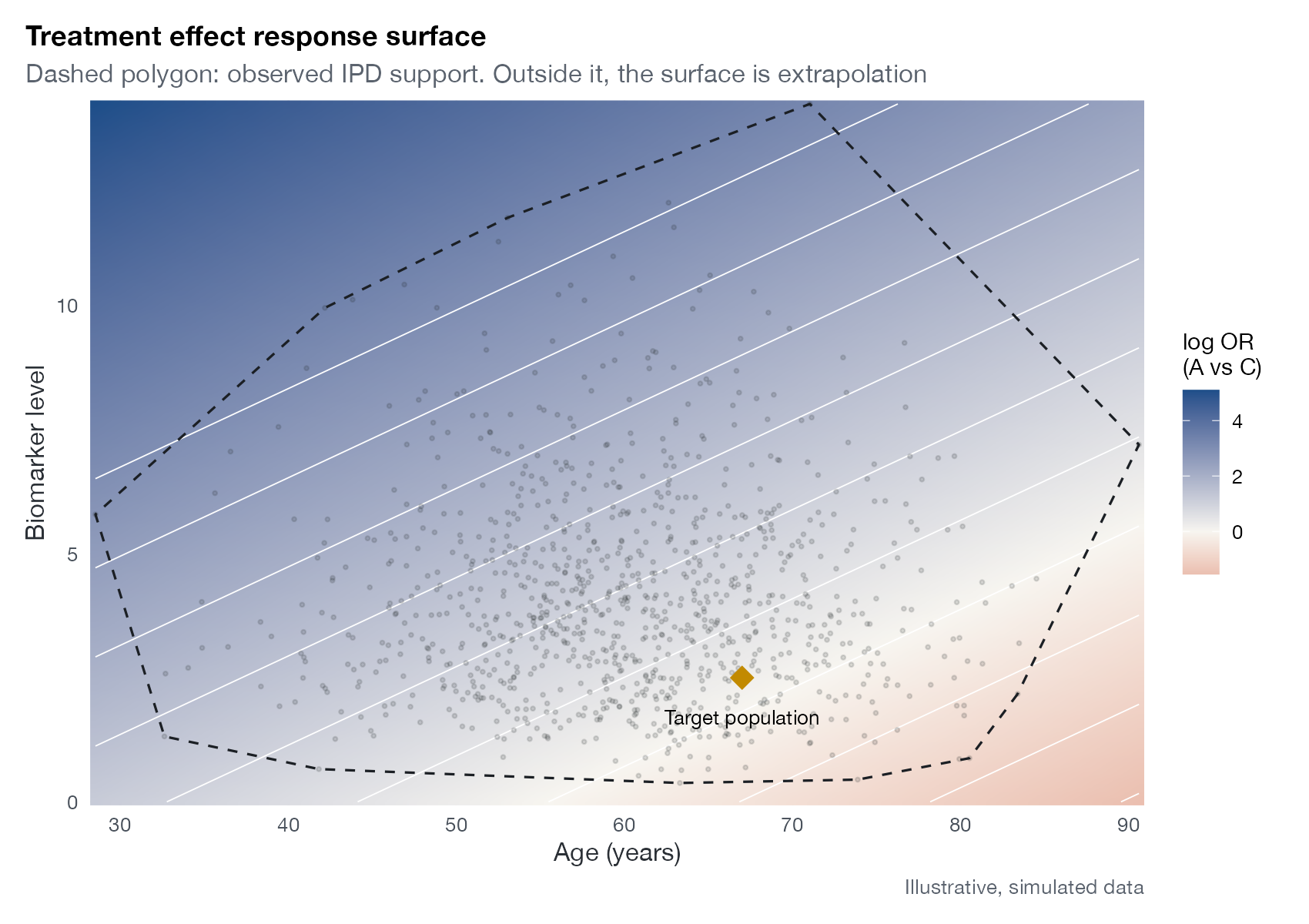
Conditional log odds ratio of A vs C from a logistic model with interactions between treatment and two continuous effect modifiers (age and a biomarker), fitted to simulated IPD. Points and the dashed convex hull show observed data; the diamond marks a target population’s means. Illustrative, simulated data.
Family
Outcome regression and transportability
Purpose
Show how the treatment effect varies jointly with two effect modifiers and where the model extrapolates.
Inputs
A fitted outcome model with at least two treatment-covariate interactions.
Software
Custom
ggplot2 (shown); plotly for interactive surfaces
What it shows
With two continuous effect modifiers, one-dimensional curves hide the joint pattern. A response surface colors the covariate plane by the predicted conditional treatment effect, with contour lines at fixed effect sizes. Overlaying the observed data and their convex hull marks where the surface is estimated from data and where it is extrapolated.
How to read it
- Axes: the two effect modifiers.
- Color: conditional treatment effect (here log OR; blue favors A).
- White contours: lines of equal effect.
- Points and dashed polygon: observed IPD and its support.
- Diamond: a target population’s covariate means.
Interpretation
The benefit of A increases with the biomarker and decreases with age. The target population, older with lower biomarker levels, sits in a region where the effect is near zero, although the average effect in the trial is clearly positive. The corners of the plane outside the dashed hull are pure extrapolation.
Pitfalls
- A smooth surface conceals uncertainty; add uncertainty slices or a standard error surface.
- Linear interaction terms force planar contours; the smoothness is an assumption, not a finding.
- A target mean inside the hull does not guarantee that the target distribution is supported.
Code
library(ggplot2)

# Simulated IPD with two continuous effect modifiers
set.seed(5)
n <- 1000
ipd <- data.frame(age = rnorm(n, 60, 9), biomarker = rgamma(n, 4, 1), trt = rep(0:1, each = n / 2))
ipd$y <- rbinom(n, 1, with(ipd, plogis(-0.5 + 0.02 * (age - 60) + 0.1 * (biomarker - 4) +
                   trt * (0.6 - 0.04 * (age - 60) + 0.25 * (biomarker - 4)))))
fit <- glm(y ~ trt * (age + biomarker), family = binomial, data = ipd)

# Conditional treatment effect (log OR) over a grid of the two modifiers
grid <- expand.grid(age = seq(min(ipd$age), max(ipd$age), length.out = 100),
                    biomarker = seq(0, max(ipd$biomarker), length.out = 100))
b <- coef(fit)
grid$logor <- b["trt"] + b["trt:age"] * grid$age + b["trt:biomarker"] * grid$biomarker
hull <- ipd[chull(ipd$age, ipd$biomarker), ]

ggplot(grid, aes(age, biomarker)) +
  geom_raster(aes(fill = logor), interpolate = TRUE) +
  geom_contour(aes(z = logor), colour = "white", breaks = seq(-2, 3, 0.5), linewidth = 0.3) +
  geom_point(data = ipd, colour = "#1b1f24", alpha = 0.15, size = 0.6) +
  geom_polygon(data = hull, fill = NA, colour = "#1b1f24", linetype = "dashed") +
  annotate("point", x = 67, y = 2.5, shape = 18, size = 5, colour = "#c28a00") +
  annotate("text", x = 67, y = 1.7, label = "Target population", size = 3.3) +
  scale_fill_gradient2(low = "#b5452b", mid = "#f7f5f0", high = "#1d4e89", midpoint = 0,
                       name = "log OR\n(A vs C)") +
  coord_cartesian(expand = FALSE) +
  labs(x = "Age (years)", y = "Biomarker level",
       title = "Treatment effect response surface",
       subtitle = "Dashed polygon: observed IPD support. Outside it, the surface is extrapolation",
       caption = "Illustrative, simulated data") +
  theme(legend.position = "right")
References
- Phillippo DM, Ades AE, Dias S, Palmer S, Abrams KR, Welton NJ. NICE DSU Technical Support Document 18: Methods for population-adjusted indirect comparisons in submissions to NICE. 2016. sheffield.ac.uk/nice-dsu
- Phillippo DM, Dias S, Ades AE, et al. Multilevel network meta-regression for population-adjusted treatment comparisons. J R Stat Soc Ser A. 2020;183:1189-1210. doi:10.1111/rssa.12579