Threshold analysis forest plot
Invariant interval plot, decision robustness plot
nmathresh example files.
nmathresh::nma_thresh() and thresh_forest()
What it shows
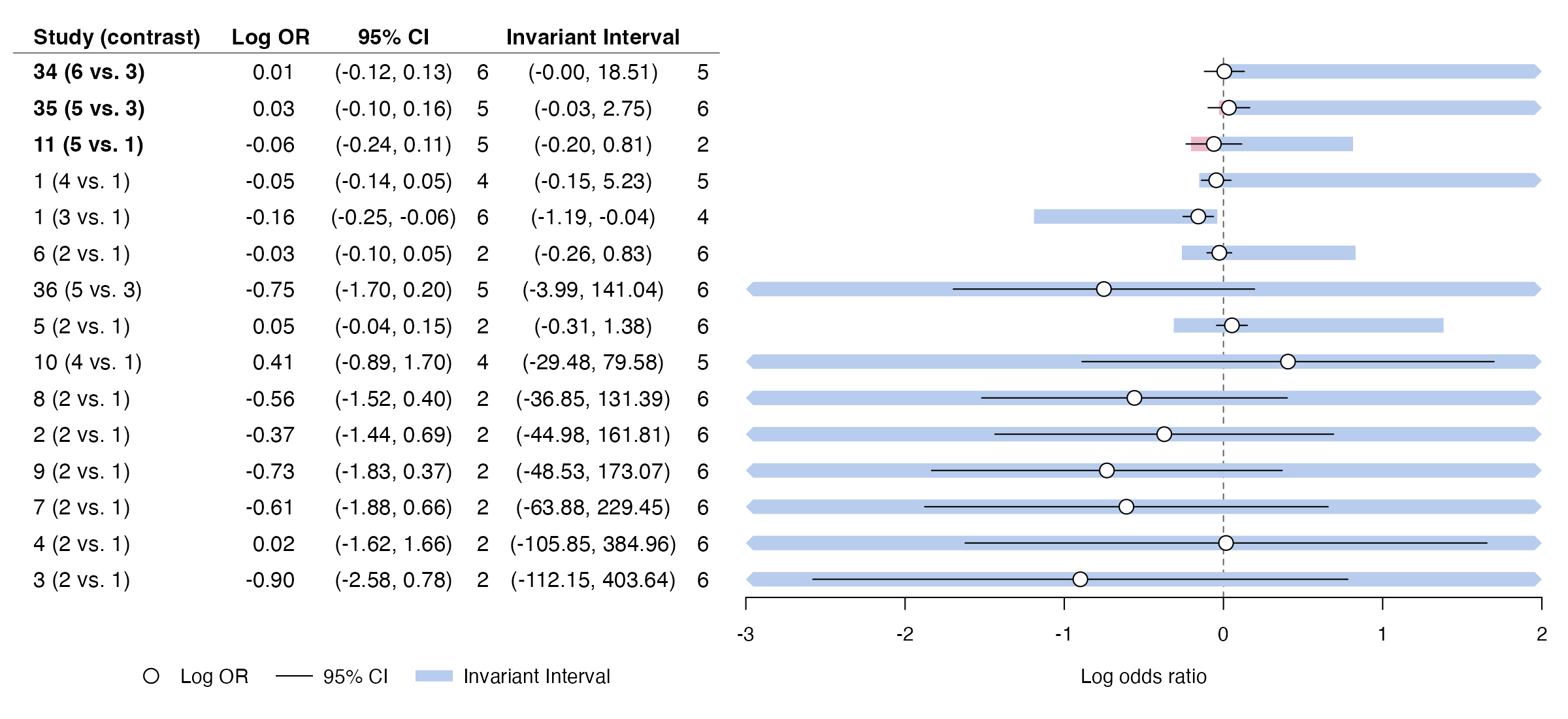
Threshold analysis (Phillippo and colleagues) asks a decision-focused question: how much could each study’s estimate change, for whatever reason, before the recommended treatment changes? The answer is an invariant interval around each data point, with the treatment that would take over at each limit. Plotting these intervals against the 95% confidence intervals shows which pieces of evidence the decision is sensitive to within the range of plausible error.
How to read it
- Rows: study contrasts, ordered by how much of the CI the invariant interval covers.
- Point and line: the study estimate and its 95% CI.
- Shaded bar: the invariant interval; within it the recommendation does not change.
- Numbers at the ends: the treatment that becomes optimal beyond each limit.
- Bold labels: contrasts whose CI extends beyond the invariant interval.
Interpretation
For most studies the invariant interval is far wider than the CI, so the recommendation (treatment 3) is robust to them. For the contrasts at the top, such as study 34 (6 vs 3), the interval barely extends below the estimate: a tiny downward adjustment would make treatment 6 optimal. Those studies deserve the closest scrutiny of risk of bias.
Pitfalls
- Thresholds assume that only one data point changes at a time; joint changes can be analyzed but are harder to display.
- The analysis is about the decision (which treatment is best), not about the estimates themselves.
- For random-effects or Bayesian models, the likelihood covariance may need to be reconstructed.
Code
library(nmathresh)
library(Matrix)

# Thrombolytics after myocardial infarction: 50 trials, 7 treatments
# (NICE DSU example; posterior summaries are bundled with nmathresh)
dat <- read.delim(system.file("extdata", "Thrombo_data.txt", package = "nmathresh"))
n <- nrow(dat)

# Log odds ratios (arm 2 vs 1, arm 3 vs 1) and their likelihood covariance
dat$lor.1 <- with(dat, log(r.2 * (n.1 - r.1) / ((n.2 - r.2) * r.1)))
dat$k.1 <- dat$t.2; dat$b.1 <- dat$t.1
dat$lor.2 <- with(dat, log(r.3 * (n.1 - r.1) / ((n.3 - r.3) * r.1)))
dat$k.2 <- dat$t.3; dat$b.2 <- ifelse(is.na(dat$k.2), NA, dat$t.1)
V <- bdiag(lapply(seq_len(n), function(i) with(dat[i, ], {
  v1 <- 1 / r.1 + 1 / r.2 + 1 / (n.1 - r.1) + 1 / (n.2 - r.2)
  if (n_arms == 2) return(v1)
  v2 <- 1 / r.1 + 1 / r.3 + 1 / (n.1 - r.1) + 1 / (n.3 - r.3)
  c1 <- 1 / r.1 + 1 / (n.1 - r.1)
  matrix(c(v1, c1, c1, v2), 2)
})))

long <- reshape(dat, varying = c("lor.1", "b.1", "k.1", "lor.2", "b.2", "k.2"),
                timevar = "c", idvar = "studyID", direction = "long")
long <- long[order(long$studyID, long$c, long$b, na.last = NA), ]
K <- length(unique(c(long$b, long$k)))
X <- t(sapply(seq_len(nrow(long)), function(i) {
  x <- rep(0, K - 1); x[long$k[i] - 1] <- 1
  if (long$b[i] != 1) x[long$b[i] - 1] <- -1
  x
}))

# How much could each study's estimate change before the recommended
# (lowest-mortality) treatment changes?
thresh <- nma_thresh(mean.dk = Thrombo.post.summary$statistics[1:(K - 1), "Mean"],
                     lhood = V, post = Thrombo.post.cov, nmatype = "fixed",
                     X = X, opt.max = FALSE)

long$lab <- paste0(long$studyID, " (", long$k, " vs. ", long$b, ")")
long$CI2.5 <- long$lor + qnorm(0.025) * sqrt(diag(V))
long$CI97.5 <- long$lor + qnorm(0.975) * sqrt(diag(V))
long$coverage <- apply(cbind(thresh$thresholds$lo / (long$CI2.5 - long$lor),
                             thresh$thresholds$hi / (long$CI97.5 - long$lor)), 1, min, na.rm = TRUE)

thresh_forest(thresh, y = lor, CI.lo = CI2.5, CI.hi = CI97.5, label = lab,
              orderby = coverage, data = long,
              CI.title = "95% CI", y.title = "Log OR", label.title = "Study (contrast)",
              xlab = "Log odds ratio", xlim = c(-3, 2), refline = 0, digits = 2,
              calcdim = FALSE)
References
- Phillippo DM, Dias S, Ades AE, Didelez V, Welton NJ. Sensitivity of treatment recommendations to bias in network meta-analysis. J R Stat Soc Ser A. 2018;181:843-867. doi:10.1111/rssa.12341
- Phillippo DM, Dias S, Welton NJ, Caldwell DM, Taske N, Ades AE. Threshold analysis as an alternative to GRADE for assessing confidence in guideline recommendations based on network meta-analyses. Ann Intern Med. 2019;170:538-546. doi:10.7326/M18-3542