Litmus Rank-O-Gram

Cumulative rankogram with SUCRA litmus strip

NMA

Cumulative rank curves colored by SUCRA, paired with a vertical color strip that places each treatment on the SUCRA scale.

NMAProposed

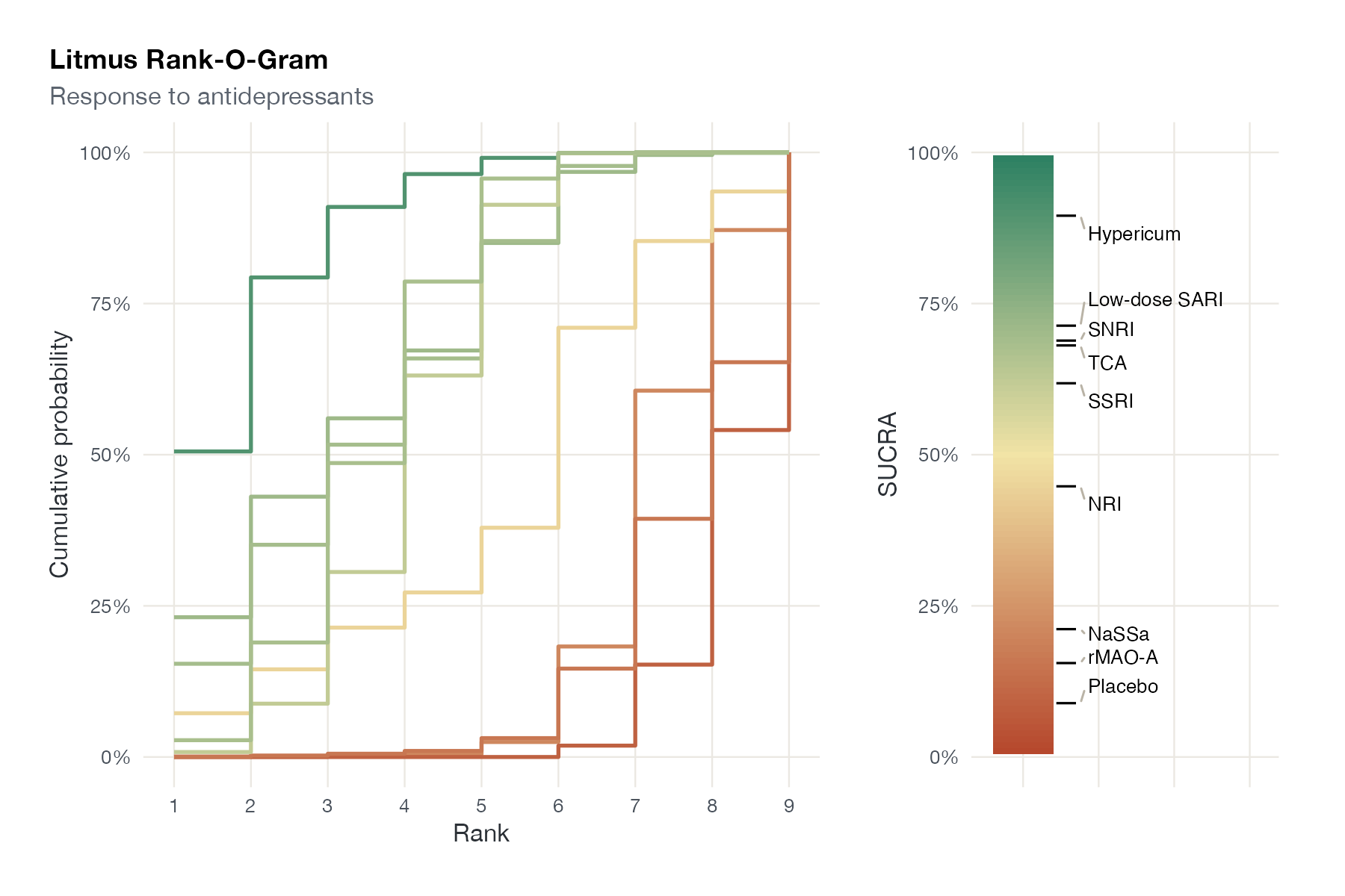
Litmus Rank-O-Gram for response in the antidepressant network: cumulative rank probabilities (left), colored by SUCRA, and a litmus strip (right) marking each treatment’s SUCRA. Custom implementation following Nevill et al. (2023). Data: netmeta::Linde2015.

Family

Treatment ranking

Purpose

Combine the full rank distributions with an at-a-glance summary.

Inputs

Cumulative rank probabilities and SUCRA values.

Software

MetaInsight web application; custom ggplot2 and patchwork (shown)

What it shows

Nevill, Cooper, and Sutton developed the Litmus Rank-O-Gram as part of a multifaceted display for network meta-analysis in the MetaInsight application. It pairs the cumulative ranking plot with a “litmus paper” strip: a color scale from red (SUCRA 0%) to green (100%) along which each treatment is marked. The curves carry the uncertainty; the strip gives the summary without hiding where it comes from.

How to read it

Left: cumulative probability of being ranked at or above each rank, one line per treatment, colored by SUCRA.
Right: SUCRA scale with each treatment marked at its value.
Close marks on the strip: treatments whose rankings are practically indistinguishable.

Interpretation

Hypericum stands alone at the top of the strip. Low-dose SARI, SNRI, and TCA sit almost on top of each other around 70%, with SSRI just below, so their order means little. NaSSa, rMAO-A, and placebo cluster near the bottom.

Pitfalls

Inherits all limitations of SUCRA.
Color alone should not carry the message; the curves must remain readable.

Code

library(netmeta)

# Antidepressants in primary care (Linde et al. 2015): arm-level binary outcomes
data(Linde2015)
d <- Linde2015
nma_for <- function(v, small) {
  p <- pairwise(treat = list(d$treatment1, d$treatment2, d$treatment3),
                event = list(d[[paste0(v, 1)]], d[[paste0(v, 2)]], d[[paste0(v, 3)]]),
                n = list(d$n1, d$n2, d$n3), studlab = d$id, sm = "OR", allstudies = TRUE)
  netmeta(p, common = FALSE, reference.group = "Placebo", small.values = small)
}
library(ggplot2)
library(patchwork)

resp <- nma_for("resp", small = "undesirable")
rk <- rankogram(resp, nsim = 5000, cumulative.rankprob = TRUE)
cm <- rk$cumrank.matrix.random
cum <- data.frame(treatment = rep(rownames(cm), ncol(cm)),
                  rank = rep(seq_len(ncol(cm)), each = nrow(cm)), p = as.vector(cm))
sucra <- data.frame(treatment = rownames(cm),
                    sucra = rowSums(cm[, -ncol(cm)]) / (ncol(cm) - 1))
pal <- colorRampPalette(c("#b5452b", "#f2e4a6", "#2a7f62"))(101)
sucra$col <- pal[round(100 * sucra$sucra) + 1]

# Cumulative rankograms, one line per treatment, colored by SUCRA
left <- ggplot(cum, aes(rank, p, group = treatment,
                        colour = sucra$col[match(treatment, sucra$treatment)])) +
  geom_step(linewidth = 0.9) +
  scale_colour_identity() +
  scale_x_continuous(breaks = 1:9) +
  scale_y_continuous(labels = scales::percent) +
  labs(x = "Rank", y = "Cumulative probability", title = "Litmus Rank-O-Gram",
       subtitle = "Response to antidepressants")

# Litmus strip: SUCRA scale with treatments placed at their SUCRA
strip <- data.frame(y = seq(0, 1, length.out = 101), col = pal)
right <- ggplot() +
  geom_tile(data = strip, aes(x = 0, y = y, fill = col), width = 0.4, height = 0.011) +
  geom_segment(data = sucra, aes(x = 0.22, xend = 0.35, y = sucra, yend = sucra)) +
  ggrepel::geom_text_repel(data = sucra, aes(x = 0.38, y = sucra, label = treatment),
                           hjust = 0, direction = "y", size = 3.3, xlim = c(0.38, NA),
                           segment.colour = "#b9b3a6", min.segment.length = 0) +
  scale_fill_identity() +
  scale_y_continuous(labels = scales::percent, limits = c(0, 1), name = "SUCRA") +
  scale_x_continuous(limits = c(-0.25, 1.6)) +
  theme(axis.text.x = element_blank(), axis.title.x = element_blank(),
        panel.grid = element_blank())

left + right + plot_layout(widths = c(2.2, 1))

References

Nevill CR, Cooper NJ, Sutton AJ. A multifaceted graphical display, including treatment ranking, was developed to aid interpretation of network meta-analysis. J Clin Epidemiol. 2023;157:83-91. doi:10.1016/j.jclinepi.2023.02.016
Linde K, Kriston L, Rücker G, et al. Efficacy and acceptability of pharmacological treatments for depressive disorders in primary care: systematic review and network meta-analysis. Ann Fam Med. 2015;13:69-79. doi:10.1370/afm.1687