Multivariate support plot
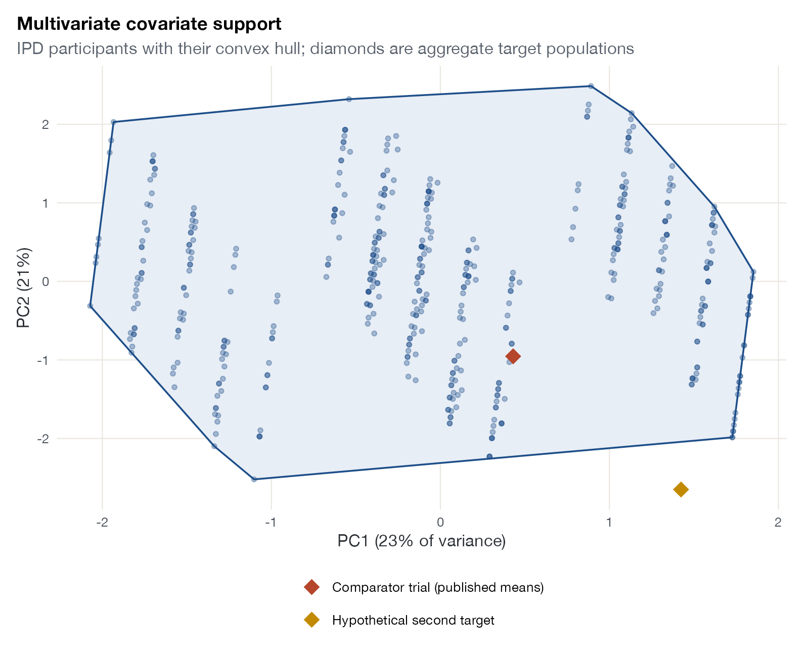
PCA convex hull plot, covariate overlap in low dimensions
maicplus::adsl_sat.
prcomp() and ggplot2 (shown)
What it shows
Population adjustment is safest when the target population lies inside the range of the IPD. Projecting the IPD onto a few principal components, drawing their convex hull, and adding the target’s covariate means gives a quick multivariate check. Outcome-regression methods (STC, G-computation, ML-NMR, ML-UMR) can extrapolate mathematically beyond the IPD where weighting cannot, so a target outside the hull is a warning that results rest on the model’s functional form.
How to read it
- Axes: the first two principal components, with the share of variance they explain.
- Points and shaded polygon: IPD participants and their convex hull.
- Diamonds: target population means projected into the same space.
Interpretation
The comparator trial’s means fall well inside the IPD cloud, so weighting or regression can reach it. The hypothetical second target, with younger, fitter, mostly male patients who rarely smoke, lies at the edge of the hull: a model would have to extrapolate to reach it.
Pitfalls
- A point inside a two-dimensional hull can still lie outside the support in the full covariate space.
- A target mean inside the hull does not mean the target distribution is supported.
- Binary covariates create striped patterns in principal components; consider other projections such as Mahalanobis distance.
- This is a suggested diagnostic, not a formal test of positivity.
Code
library(ggplot2)

data(adsl_sat, package = "maicplus")
ipd <- adsl_sat[, c("AGE", "SEX_MALE", "ECOG0", "SMOKE", "N_PR_THER")]

# Principal components of the IPD covariates
pca <- prcomp(ipd, scale. = TRUE)
scores <- as.data.frame(pca$x[, 1:2])
hull <- scores[chull(scores), ]

# Project two aggregate-data target populations (means) into the same space
targets <- data.frame(
  label = c("Comparator trial (published means)", "Hypothetical second target"),
  AGE = c(51, 38), SEX_MALE = c(0.49, 0.85), ECOG0 = c(0.35, 0.95),
  SMOKE = c(0.19, 0.02), N_PR_THER = c(2, 0.2)
)
tp <- cbind(targets["label"], predict(pca, targets[, colnames(ipd)])[, 1:2])
var <- round(100 * pca$sdev^2 / sum(pca$sdev^2))

ggplot(scores, aes(PC1, PC2)) +
  geom_polygon(data = hull, fill = "#e8eef6", colour = "#1d4e89", linewidth = 0.6) +
  geom_point(colour = "#1d4e89", alpha = 0.35, size = 1.3) +
  geom_point(data = tp, aes(colour = label), size = 5, shape = 18) +
  scale_colour_manual(values = c("#b5452b", "#c28a00"), name = NULL) +
  labs(x = sprintf("PC1 (%d%% of variance)", var[1]), y = sprintf("PC2 (%d%%)", var[2]),
       title = "Multivariate covariate support",
       subtitle = "IPD participants with their convex hull; diamonds are aggregate target populations") +
  guides(colour = guide_legend(ncol = 1))
References
- Phillippo DM, Ades AE, Dias S, Palmer S, Abrams KR, Welton NJ. NICE DSU Technical Support Document 18: Methods for population-adjusted indirect comparisons in submissions to NICE. 2016. sheffield.ac.uk/nice-dsu
- King G, Zeng L. The dangers of extreme counterfactuals. Polit Anal. 2006;14:131-159. doi:10.1093/pan/mpj004