Dose-response meta-analysis plot
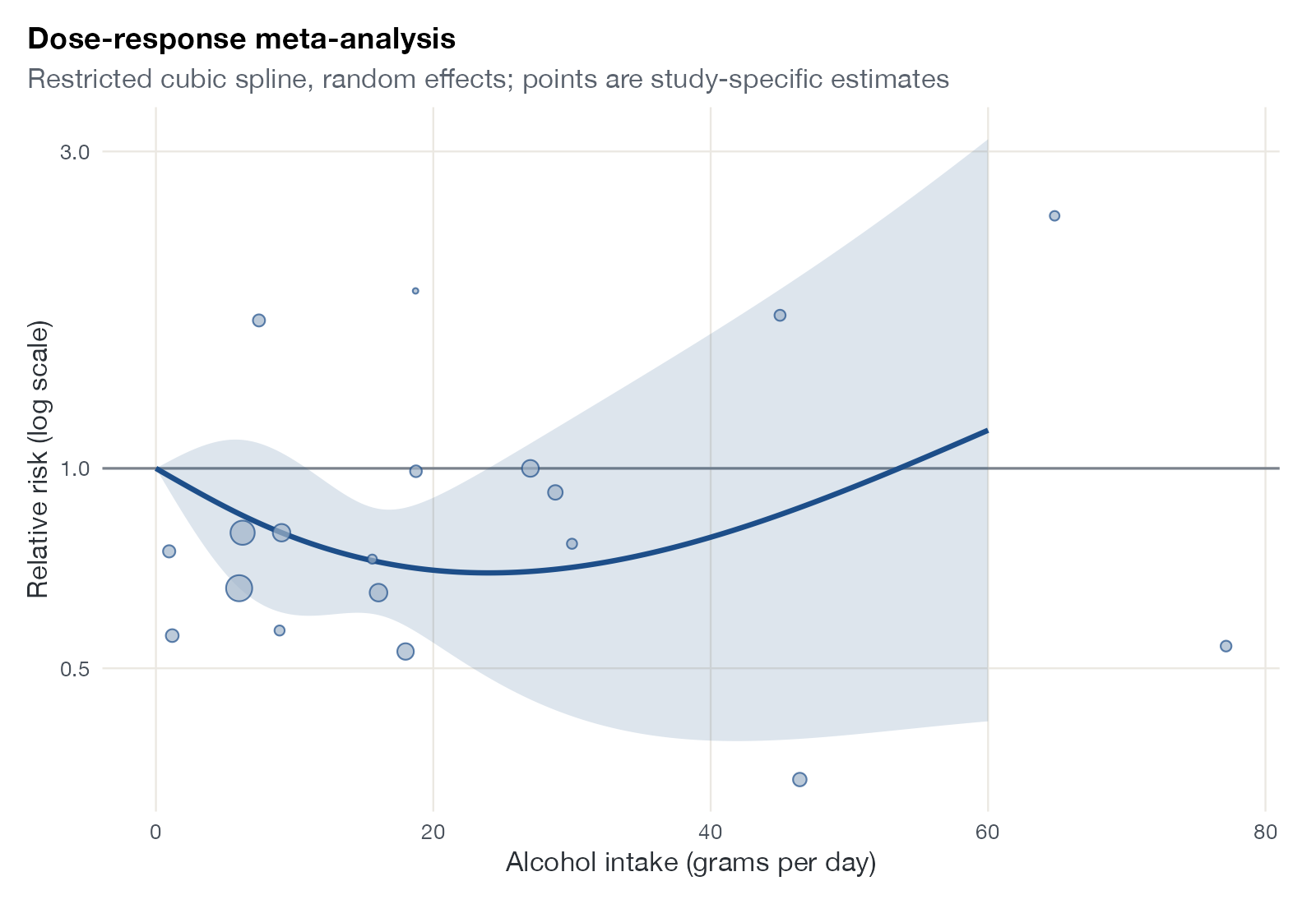
Pooled dose-response curve
dosresmeta::alcohol_cvd.
dosresmeta, metafor; Stata drmeta
What it shows
Many studies report effects for several exposure categories against a reference level. Dose-response meta-analysis (Greenland and Longnecker; Orsini and colleagues) accounts for the correlation between estimates that share a reference group and pools the within-study dose-response curves. Flexible shapes, such as restricted cubic splines, reveal nonlinear relationships like thresholds and J-shapes.
How to read it
- Horizontal axis: dose or exposure.
- Vertical axis: relative risk against the reference dose, on a log scale.
- Curve and band: pooled dose-response relationship and 95% CI.
- Points: study-specific estimates at each dose.
Interpretation
The pooled curve is J-shaped: risk falls to about 0.7 at roughly 20 to 30 grams per day and returns to 1 near 50 grams, with wide uncertainty at higher intakes where data are sparse. The lower risk at moderate intake is the kind of finding for which residual confounding and reference-group choice matter more than the curve’s shape.
Pitfalls
- Observational dose-response relationships inherit confounding from the primary studies.
- Spline knots and the reference dose influence the shape; report them and consider sensitivity analyses.
- Assigned doses within open-ended categories are assumptions.
Code
library(dosresmeta)
library(rms)
library(ggplot2)

# Alcohol intake and cardiovascular disease risk: 8 cohort studies
data(alcohol_cvd)

# Two-stage random-effects dose-response meta-analysis with restricted cubic splines
k <- quantile(alcohol_cvd$dose, c(0.05, 0.35, 0.65, 0.95))
spl <- dosresmeta(formula = logrr ~ rcs(dose, k), type = type, id = id,
                  se = se, cases = cases, n = n, data = alcohol_cvd)

newd <- data.frame(dose = seq(0, 60, length.out = 200))
pred <- predict(spl, newdata = newd, expo = TRUE)
pred$dose <- newd$dose

ggplot(pred, aes(dose, pred)) +
  geom_hline(yintercept = 1, colour = "#7a828c") +
  geom_ribbon(aes(ymin = ci.lb, ymax = ci.ub), fill = "#1d4e89", alpha = 0.15) +
  geom_line(colour = "#1d4e89", linewidth = 1.1) +
  geom_point(data = subset(alcohol_cvd, se > 0), aes(dose, exp(logrr), size = 1 / se^2),
             inherit.aes = FALSE, shape = 21, fill = "#9fb3c8", colour = "#1d4e89", alpha = 0.7) +
  scale_size_area(max_size = 5, guide = "none") +
  scale_y_log10() +
  labs(x = "Alcohol intake (grams per day)", y = "Relative risk (log scale)",
       title = "Dose-response meta-analysis",
       subtitle = "Restricted cubic spline, random effects; points are study-specific estimates")
References
- Greenland S, Longnecker MP. Methods for trend estimation from summarized dose-response data, with applications to meta-analysis. Am J Epidemiol. 1992;135:1301-1309. doi:10.1093/oxfordjournals.aje.a116237
- Crippa A, Orsini N. Multivariate dose-response meta-analysis: the dosresmeta R package. J Stat Softw. 2016;72(Code Snippet 1):1-15. doi:10.18637/jss.v072.c01