Q decomposition plot
Design-by-treatment decomposition of Cochran’s Q
NMA
Cochran’s Q split into within-design heterogeneity and between-design inconsistency, with the contribution of each design.
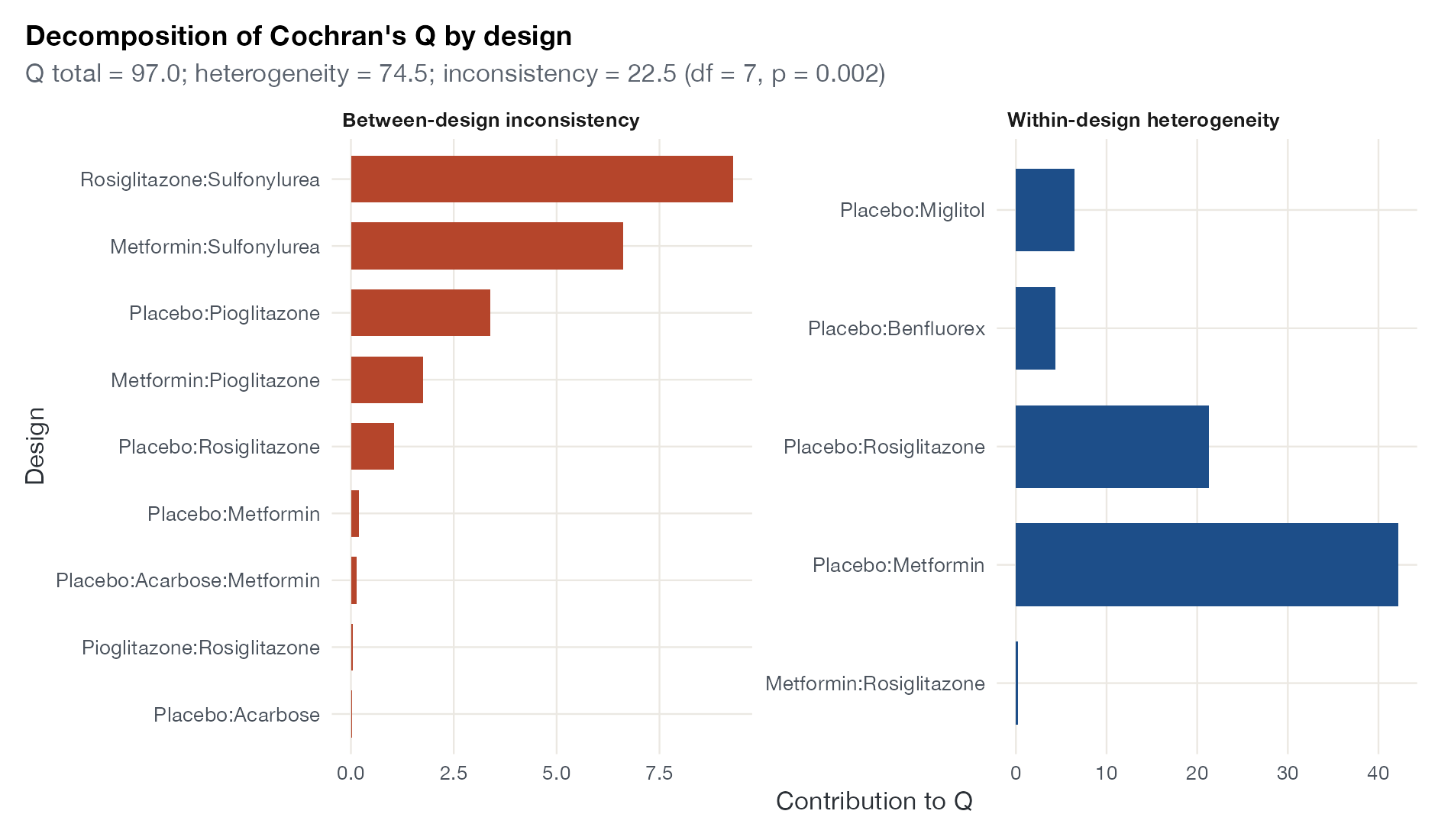
Decomposition of Cochran’s Q for the diabetes network (common-effect model) into within-design heterogeneity and between-design inconsistency, with each design’s contribution. Data:
netmeta::Senn2013.
Family
Inconsistency
Purpose
Separate heterogeneity from inconsistency and see which designs contribute to each.
Inputs
A fitted network meta-analysis.
Software
R
netmeta::decomp.design() with ggplot2; Stata network meta inconsistency
What it shows
The total Cochran’s Q of a network meta-analysis can be split into two parts (Krahn and colleagues): heterogeneity among studies of the same design, and inconsistency between designs, which corresponds to the design-by-treatment interaction model of Higgins and colleagues. Plotting each design’s contribution to both parts shows where the global signal comes from.
How to read it
- Right panel: contribution of each design to within-design heterogeneity.
- Left panel: contribution of each design to between-design inconsistency (from detaching it).
- Subtitle: total, heterogeneity, and inconsistency Q with the global test of inconsistency.
Interpretation
Total Q is 97.0, of which 74.5 is heterogeneity within designs (mostly among the metformin and rosiglitazone versus placebo trials) and 22.5 is inconsistency between designs (df = 7, \(p = 0.002\)). The inconsistency is concentrated in the two sulfonylurea comparisons, in line with the net heat plot.
Pitfalls
- A non-significant global test does not prove consistency; it has low power.
- Under a common-effect model, heterogeneity inflates the inconsistency test; random-effects versions are also available.
- Contributions of detached designs are not additive.
Code
library(netmeta)
library(ggplot2)

data(Senn2013)

net <- netmeta(
  TE, seTE, treat1.long, treat2.long, studlab,
  data = Senn2013, sm = "MD",
  common = TRUE, reference.group = "Placebo"
)

# Decompose Cochran's Q into within-design heterogeneity and
# between-design inconsistency, and show each design's contribution
dd <- decomp.design(net)
het <- dd$Q.het.design
inc <- dd$Q.inc.design
d <- rbind(
  data.frame(design = het$design, Q = het$Q, part = "Within-design heterogeneity"),
  data.frame(design = names(inc), Q = as.numeric(inc), part = "Between-design inconsistency")
)
d <- d[d$Q > 0.01, ]
d$design <- factor(d$design, levels = unique(d$design[order(d$Q)]))

ggplot(d, aes(Q, design, fill = part)) +
  geom_col(width = 0.7) +
  facet_wrap(~ part, scales = "free") +
  scale_fill_manual(values = c("#b5452b", "#1d4e89"), guide = "none") +
  labs(x = "Contribution to Q", y = "Design",
       title = "Decomposition of Cochran's Q by design",
       subtitle = sprintf("Q total = %.1f; heterogeneity = %.1f; inconsistency = %.1f (df = %d, p = %.3f)",
                          dd$Q.decomp$Q[1], dd$Q.decomp$Q[2], dd$Q.decomp$Q[3],
                          dd$Q.decomp$df[3], dd$Q.decomp$pval[3]))
References
- Krahn U, Binder H, König J. A graphical tool for locating inconsistency in network meta-analyses. BMC Med Res Methodol. 2013;13:35. doi:10.1186/1471-2288-13-35
- Higgins JPT, Jackson D, Barrett JK, Lu G, Ades AE, White IR. Consistency and inconsistency in network meta-analysis: concepts and models for multi-arm studies. Res Synth Methods. 2012;3:98-110. doi:10.1002/jrsm.1044