Heterogeneity profile likelihood plot
Profile likelihood for tau², likelihood profile plot
metadat::dat.bcg.
metafor::profile(), metafor::confint()
What it shows
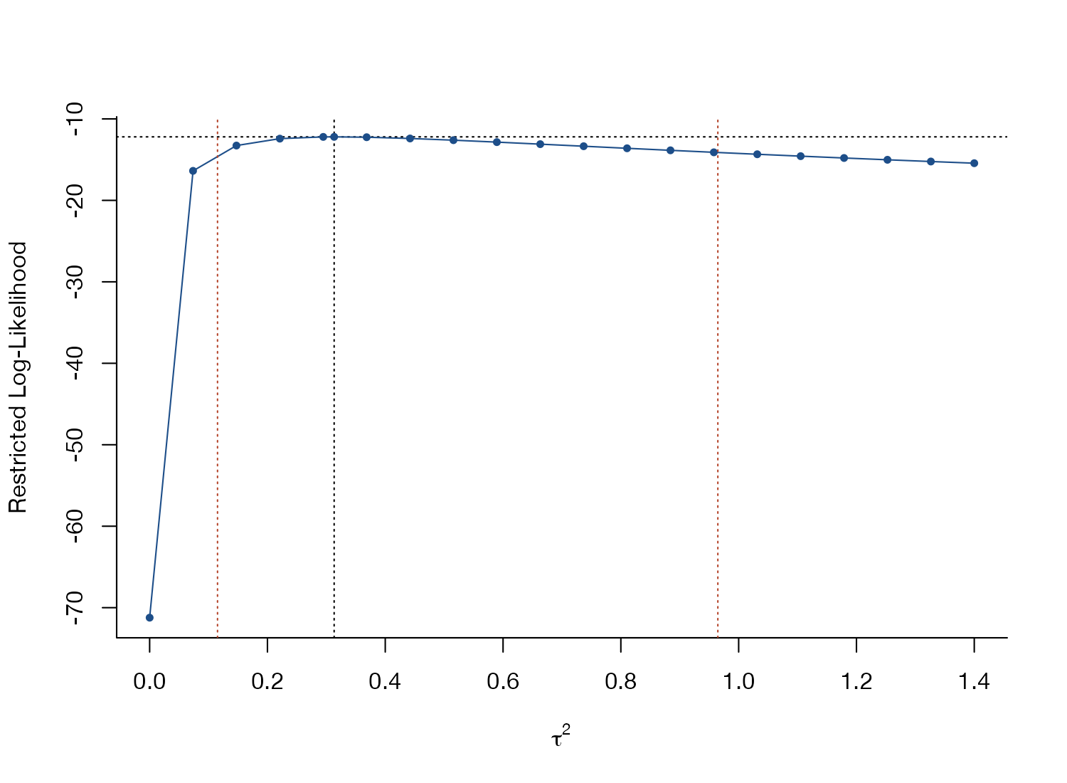
Heterogeneity is usually summarized by a single number, \(\hat\tau^2\) or \(I^2\), but it is often poorly estimated. The profile plot traces the (restricted) log-likelihood over a grid of \(\tau^2\) values, maximizing over the other parameters at each point. A sharp peak means the data identify \(\tau^2\) well; a flat ridge means they do not. The interval where the curve lies within 1.92 units of its maximum is the 95% profile-likelihood confidence interval.
How to read it
- Horizontal axis: \(\tau^2\).
- Vertical axis: restricted log-likelihood.
- Peak: the REML estimate.
- Flatness: how weakly the data inform \(\tau^2\).
- Vertical lines (added here): the profile-likelihood confidence limits.
Interpretation
The curve has a clear maximum at \(\hat\tau^2 = 0.31\), but it is flat to the right: values up to about 0.96 are compatible with the data. The corresponding \(I^2\) interval runs from 81% to 97%. The heterogeneity is certainly large, but its size is uncertain by a factor of about eight, which carries over to the width of the prediction interval.
Pitfalls
- A flat profile, or a maximum at the boundary \(\tau^2 = 0\), signals that heterogeneity is not identifiable from the data; the reported \(\hat\tau^2\) then means little.
- In multilevel or multivariate models, profile every variance component; one may be unidentified while others are fine.
- Different estimators (DL, REML, PM) give different point estimates; the profile shows the REML objective only.
Code
library(metafor)

data(dat.bcg, package = "metadat")
dat <- escalc(measure = "RR", ai = tpos, bi = tneg, ci = cpos, di = cneg,
              data = dat.bcg)

fit <- rma(yi, vi, data = dat, method = "REML")

# Restricted log-likelihood as a function of tau^2, with the REML estimate
# and a 95% profile-likelihood confidence interval
ci <- confint(fit, type = "PL")
profile(fit, xlim = c(0, 1.4), col = "#1d4e89", pch = 19, cex = 0.6,
        main = "", xlab = expression(tau^2))
abline(v = ci$random["tau^2", c("ci.lb", "ci.ub")], lty = "dotted", col = "#b5452b")
References
- Viechtbauer W. Confidence intervals for the amount of heterogeneity in meta-analysis. Stat Med. 2007;26:37-52. doi:10.1002/sim.2514
- Hardy RJ, Thompson SG. A likelihood approach to meta-analysis with random effects. Stat Med. 1996;15:619-629. doi:10.1002/(SICI)1097-0258(19960330)15:6<619::AID-SIM188>3.0.CO;2-A