Proportional hazards diagnostic plots
Log cumulative hazard plot, Schoenfeld residual plot
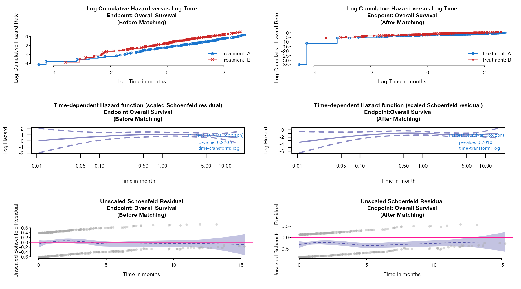
maicplus examples.
maicplus::ph_diagplot(), survival::cox.zph(); Stata estat phtest, stphplot
What it shows
Many syntheses of survival outcomes pool or compare hazard ratios, which assumes that hazards are proportional over time. Two classic diagnostics test that assumption. If hazards are proportional, curves of log cumulative hazard against log time run parallel. The scaled Schoenfeld residuals estimate the log hazard ratio as a function of time; a flat line supports proportionality, and the Grambsch-Therneau test gives a p-value. NICE DSU TSD 14 recommends these checks before any hazard ratio is used.
How to read it
- Top: log cumulative hazard against log time for each arm; look for parallel curves.
- Middle: smoothed time-varying log hazard ratio with confidence band; look for a flat line.
- Bottom: unscaled residuals with a smoother.
- Left and right panels: before and after MAIC weighting.
Interpretation
The log cumulative hazard curves are roughly parallel, and the Schoenfeld test does not reject proportional hazards before (p = 0.82) or after weighting (p = 0.70). A hazard ratio is a reasonable summary here, although the tests have limited power and the curves diverge slightly at early times.
Pitfalls
- A non-significant test is not proof of proportional hazards; look at the shape.
- Log cumulative hazard plots are sensitive to small numbers at the extremes of follow-up.
- In NMA, proportional hazards must hold for every comparison; violations call for time-varying models (see the time-varying hazard ratio plot).
Code
library(maicplus)

data(weighted_sat)
data(adtte_sat)
data(pseudo_ipd_sat)

# Log cumulative hazard against log time (parallel curves support
# proportional hazards), and scaled Schoenfeld residuals over time
ph_diagplot(
  weights_object = weighted_sat,
  tte_ipd = adtte_sat, tte_pseudo_ipd = pseudo_ipd_sat,
  trt_var_ipd = "ARM", trt_var_agd = "ARM",
  trt_ipd = "A", trt_agd = "B",
  endpoint_name = "Overall Survival",
  time_scale = "month", zph_transform = "log", zph_log_hazard = TRUE
)
References
- Grambsch PM, Therneau TM. Proportional hazards tests and diagnostics based on weighted residuals. Biometrika. 1994;81:515-526. doi:10.1093/biomet/81.3.515
- Latimer NR. NICE DSU Technical Support Document 14: Survival analysis for economic evaluations alongside clinical trials, extrapolation with patient-level data. 2011, updated 2013. sheffield.ac.uk/nice-dsu