Leverage versus residual deviance plot

Leverage plot, DIC contribution plot

NMA

ML-NMR

Each data point’s leverage against its signed Bayesian deviance residual, with contours of its contribution to the DIC.

Leverage against signed square-root residual deviance for each arm in a Bayesian random-effects NMA of 24 smoking cessation trials. Curves mark leverage plus squared residual equal to 1, 2, 3, and 4; points outside the outer curves contribute most to the DIC. Data: multinma::smoking.

Family

Model checking and Bayesian diagnostics

Purpose

Identify data points that fit poorly or strongly influence the model in Bayesian evidence synthesis.

Inputs

Posterior mean residual deviance and leverage for every data point.

Software

R multinma::plot(dic(), type = "leverage"); BUGS or JAGS output with custom plots

What it shows

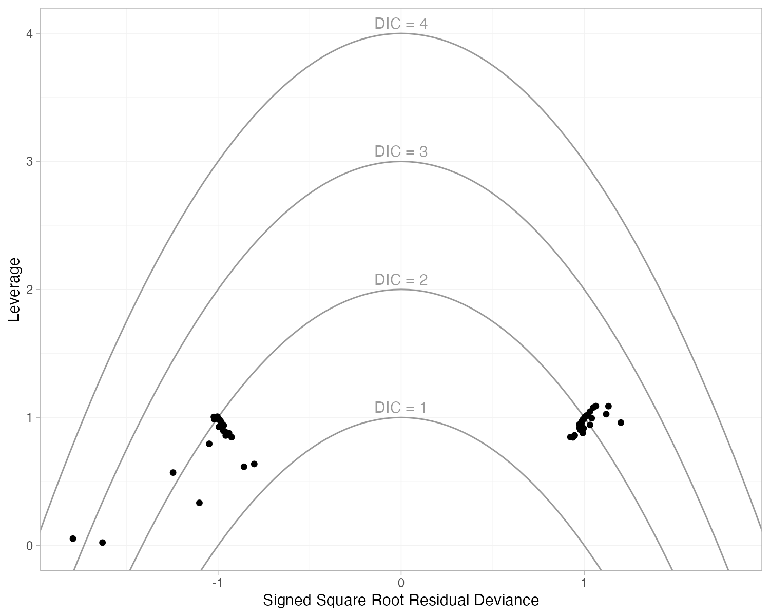
The NICE Decision Support Unit’s Technical Support Document 2 recommends this plot for Bayesian pairwise and network meta-analysis. For each data point (an arm, or a contrast), the posterior mean residual deviance measures lack of fit and the leverage \(p_{D,i}\) measures how much the point pulls its own fitted value. Plotting leverage against the signed square root of the residual deviance, with parabolas where leverage plus squared residual is constant, shows which points contribute most to the deviance information criterion.

How to read it

Horizontal axis: signed \(\sqrt{\text{residual deviance}}\); negative when the observed value is below the fitted value.
Vertical axis: leverage.
Curves: \(\text{leverage} + \text{residual}^2 = c\) for \(c = 1, 2, 3, 4\); points beyond \(c = 3\) are generally considered to contribute to poor fit.
Clusters near ±1 with leverage near 1: typical of random-effects models, where each arm is fitted almost exactly.

Interpretation

Total residual deviance is 54 against 50 data points, which indicates adequate fit. Most arms sit near \((\pm 1, 1)\). A few points lie between the second and third curves, such as the no-intervention arm of study 15, which observed zero quitters when 1.5 were expected. None lies far outside, so no single arm dominates the DIC.

Pitfalls

The residual deviance per data point should be about 1 under a good fit; compare totals with the number of data points, not with zero.
Leverage depends on the model; random-effects models have high leverage almost everywhere.
A poorly fitting point is a prompt to check data extraction and clinical differences, not an automatic exclusion.

Code

library(multinma)

# Smoking cessation: 24 trials of four interventions (NICE DSU TSD 2)
net <- set_agd_arm(smoking, study = studyn, trt = trtc, r = r, n = n,
                   trt_ref = "No intervention")

fit <- nma(net, trt_effects = "random",
           prior_intercept = normal(scale = 100),
           prior_trt = normal(scale = 100),
           prior_het = half_normal(scale = 5),
           seed = 2026)

# Leverage against Bayesian deviance residual, with contours of
# leverage + residual^2 = 1, 2, 3, 4 (each data point's contribution to DIC)
plot(dic(fit), type = "leverage")

References

Dias S, Welton NJ, Sutton AJ, Ades AE. NICE DSU Technical Support Document 2: A generalised linear modelling framework for pairwise and network meta-analysis of randomised controlled trials. 2011, updated 2016. NCBI Bookshelf NBK310366
Spiegelhalter DJ, Best NG, Carlin BP, van der Linde A. Bayesian measures of model complexity and fit. J R Stat Soc Ser B. 2002;64:583-639. doi:10.1111/1467-9868.00353
Phillippo DM. multinma: Bayesian network meta-analysis of individual and aggregate data. R package. dmphillippo.github.io/multinma