MCMC trace, rank, and density plots
Convergence diagnostics
multinma::smoking.
bayesplot::mcmc_trace(), mcmc_rank_overlay(), mcmc_dens_overlay(); Python arviz
What it shows
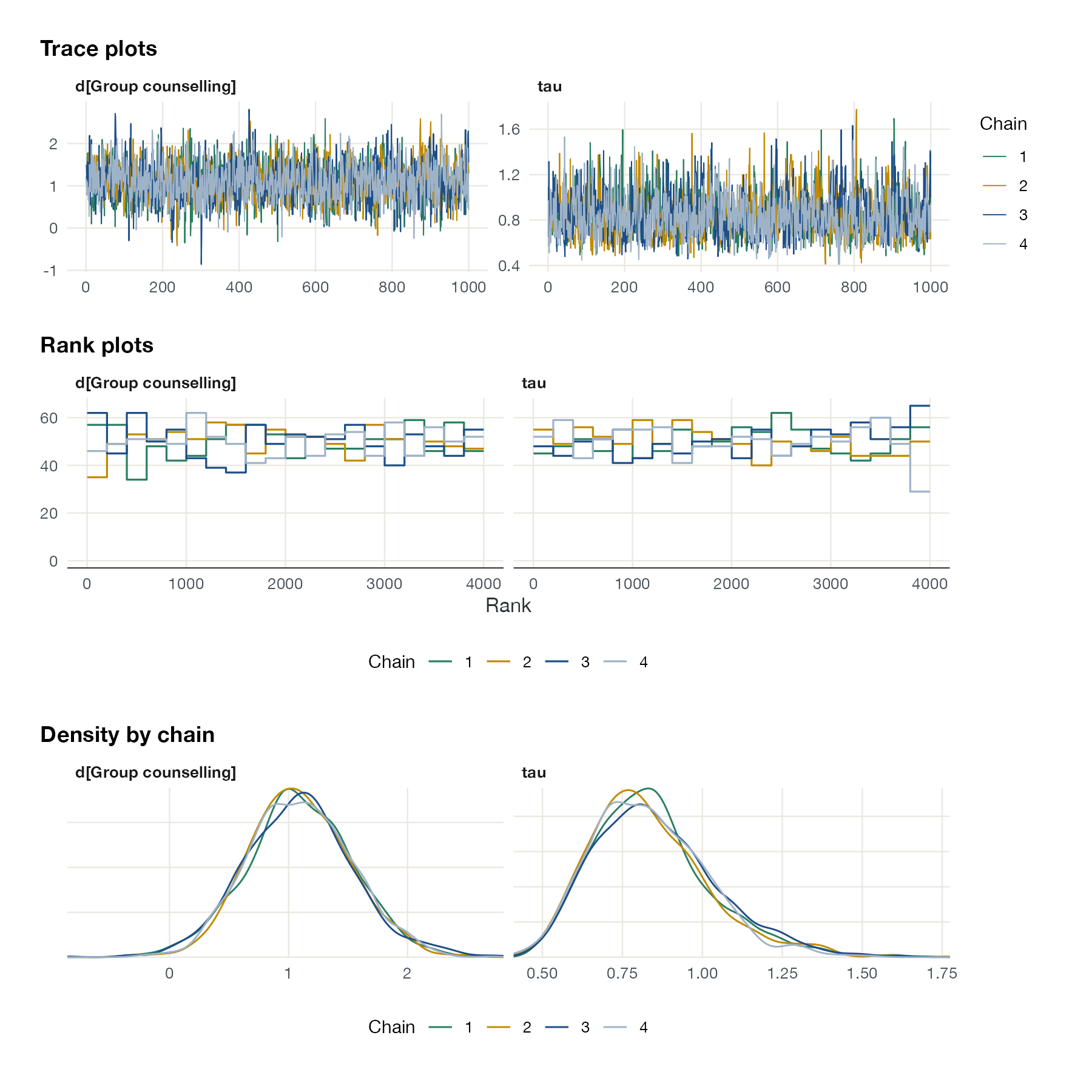
Every Bayesian NMA, ML-NMR, ML-UMR, or Bayesian STC relies on Markov chain Monte Carlo. Three complementary plots check that the sampler worked. Trace plots show the sampled value by iteration for each chain; well-mixed chains look like overlapping “hairy caterpillars”. Rank plots rank all draws jointly and show each chain’s histogram of ranks; uniform, overlapping histograms indicate good mixing and are more sensitive than trace plots. Per-chain densities should coincide.
How to read it
- Trace plots: iteration on the horizontal axis, sampled value on the vertical; look for stationarity and overlap.
- Rank plots: each chain’s rank histogram drawn as a line; they should be flat and overlapping.
- Density by chain: each chain’s posterior density; they should agree.
- Pair with numbers: \(\hat R\) below 1.01 and adequate effective sample sizes.
Interpretation
All four chains overlap in every panel, rank histograms are flat, and densities agree, including for the heterogeneity SD \(\tau\), which is often the hardest parameter to sample. \(\hat R \le 1.01\) and bulk effective sample sizes exceed 1,000 for all treatment effects and \(\tau\).
Pitfalls
- Convergence diagnostics check the computation, not the model. A perfectly converged sampler can estimate a badly misspecified model very precisely.
- Trace plots of a few parameters can hide problems elsewhere; check \(\hat R\) and ESS for all parameters, and divergent transitions for HMC.
- Heterogeneity parameters near zero and weakly identified interactions are where problems usually appear.
Code
library(multinma)
library(bayesplot)
library(patchwork)

net <- set_agd_arm(smoking, study = studyn, trt = trtc, r = r, n = n,
                   trt_ref = "No intervention")

fit <- nma(net, trt_effects = "random",
           prior_intercept = normal(scale = 100),
           prior_trt = normal(scale = 100),
           prior_het = half_normal(scale = 5),
           seed = 2026)

draws <- as.array(fit, pars = c("d", "tau"))
color_scheme_set(c("#9fb3c8", "#5f82ab", "#1d4e89", "#b5452b", "#c28a00", "#2a7f62"))

trace <- mcmc_trace(draws, pars = c("d[Group counselling]", "tau")) +
  ggplot2::labs(title = "Trace plots")
rank <- mcmc_rank_overlay(draws, pars = c("d[Group counselling]", "tau")) +
  ggplot2::labs(title = "Rank plots")
dens <- mcmc_dens_overlay(draws, pars = c("d[Group counselling]", "tau")) +
  ggplot2::labs(title = "Density by chain")

trace / rank / dens
import arviz as az
az.plot_trace(idata, var_names=["d", "tau"])
az.plot_rank(idata, var_names=["d", "tau"])
print(az.summary(idata, var_names=["d", "tau"]))References
- Vehtari A, Gelman A, Simpson D, Carpenter B, Bürkner PC. Rank-normalization, folding, and localization: an improved R-hat for assessing convergence of MCMC. Bayesian Anal. 2021;16:667-718. doi:10.1214/20-BA1221
- Gabry J, Simpson D, Vehtari A, Betancourt M, Gelman A. Visualization in Bayesian workflow. J R Stat Soc Ser A. 2019;182:389-402. doi:10.1111/rssa.12378