Weighted covariate distribution plot

Weighted density or ECDF plot

MAIC

The distribution of a covariate in the IPD before and after weighting, against the distribution assumed for the comparator population.

MAICAdapted

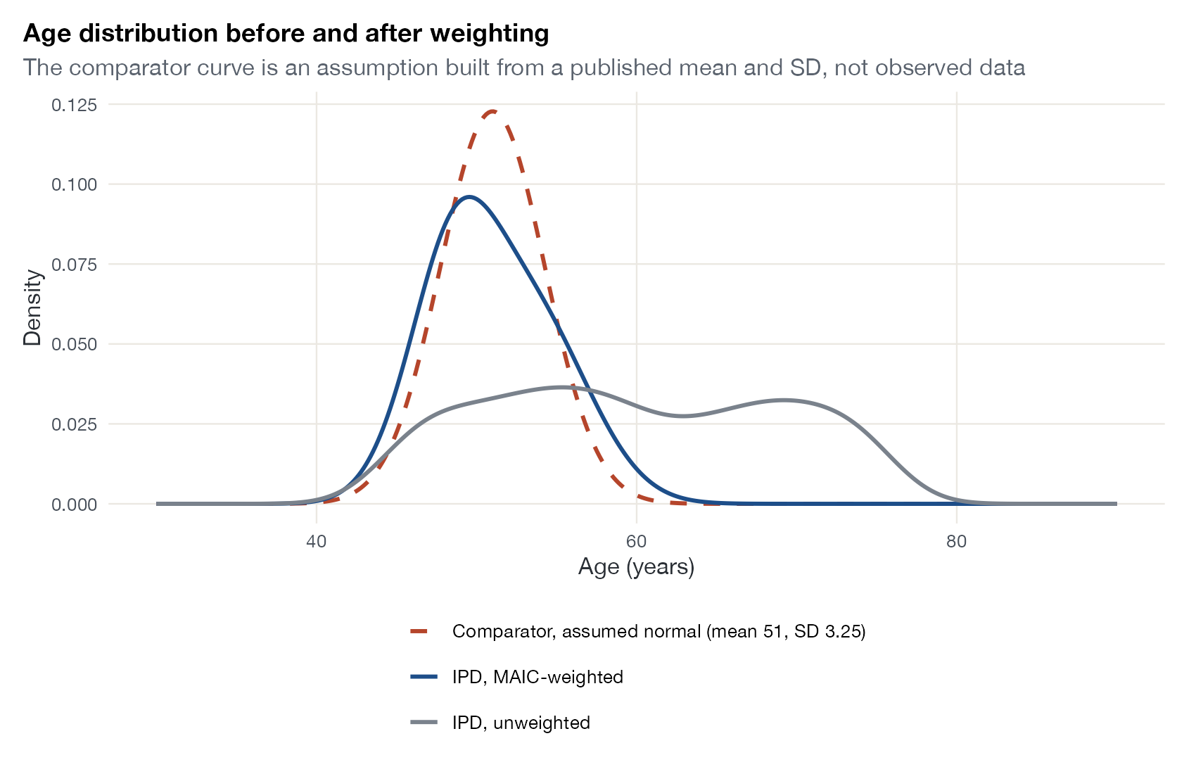
Age distribution of simulated IPD before (gray) and after (blue) MAIC weighting that matches the comparator’s mean and SD of age, against a normal distribution built from the published mean and SD (red, dashed). Data: maicplus::centered_ipd_sat.

Family

Weighting, balance, and overlap

Purpose

Show how weighting reshapes the whole covariate distribution, not just its mean.

Inputs

IPD covariate values, MAIC weights, and published summary statistics.

Software

Custom ggplot2 with weighted densities or ECDFs

What it shows

A Love plot compares means. This plot compares whole distributions: the covariate’s density (or empirical cumulative distribution) in the IPD before and after weighting, with the comparator population overlaid where it is known. It exposes tails, skewness, and multimodality that matched means conceal.

How to read it

Horizontal axis: the covariate.
Gray curve: unweighted IPD.
Blue curve: MAIC-weighted IPD.
Red dashed curve: the comparator distribution, here only an assumption built from a published mean and SD.

Interpretation

The IPD ages are broad and bimodal, spanning roughly 40 to 80. Matching both the mean (51) and SD (3.25) of the comparator squeezes the weighted distribution into a narrow peak around 45 to 57 years; 97% of the total weight falls on the 222 participants in that range. The weighted curve still differs in shape from the assumed normal target, a reminder that matching two moments does not reproduce a distribution.

Pitfalls

When only a mean and SD are published, any drawn comparator distribution is an assumption, not data. Label it as such.
Weighted densities depend on the bandwidth; very concentrated weights produce spiky curves.
Show the covariates that matter most clinically, not only those that look well balanced.

Code

library(maicplus)
library(ggplot2)

# Weights that match the comparator's mean AND SD of age (plus sex, ECOG,
# smoking, and number of prior therapies), from the maicplus example
data(centered_ipd_sat)
cc <- grep("_CENTERED$", names(centered_ipd_sat), value = TRUE)
ipd <- estimate_weights(centered_ipd_sat, centered_colnames = cc)$data

grid <- seq(30, 90, length.out = 400)
dens <- function(w) density(ipd$AGE, weights = w / sum(w), bw = 2.5, from = 30, to = 90, n = 400)$y
d <- rbind(
  data.frame(age = grid, y = dens(rep(1, nrow(ipd))), what = "IPD, unweighted"),
  data.frame(age = grid, y = dens(ipd$weights), what = "IPD, MAIC-weighted"),
  data.frame(age = grid, y = dnorm(grid, 51, 3.25), what = "Comparator, assumed normal (mean 51, SD 3.25)")
)

ggplot(d, aes(age, y, colour = what, linetype = what)) +
  geom_line(linewidth = 1) +
  scale_colour_manual(values = c("IPD, unweighted" = "#7a828c", "IPD, MAIC-weighted" = "#1d4e89",
                                 "Comparator, assumed normal (mean 51, SD 3.25)" = "#b5452b"),
                      name = NULL) +
  scale_linetype_manual(values = c("IPD, unweighted" = "solid", "IPD, MAIC-weighted" = "solid",
                                   "Comparator, assumed normal (mean 51, SD 3.25)" = "dashed"),
                        name = NULL) +
  labs(x = "Age (years)", y = "Density",
       title = "Age distribution before and after weighting",
       subtitle = "The comparator curve is an assumption built from a published mean and SD, not observed data") +
  guides(colour = guide_legend(ncol = 1), linetype = guide_legend(ncol = 1))

References

Phillippo DM, Ades AE, Dias S, Palmer S, Abrams KR, Welton NJ. NICE DSU Technical Support Document 18: Methods for population-adjusted indirect comparisons in submissions to NICE. 2016. sheffield.ac.uk/nice-dsu
Remiro-Azócar A, Heath A, Baio G. Methods for population adjustment with limited access to individual patient data: a review and simulation study. Res Synth Methods. 2021;12:750-775. doi:10.1002/jrsm.1511