GOSH plot
Graphical display of study heterogeneity
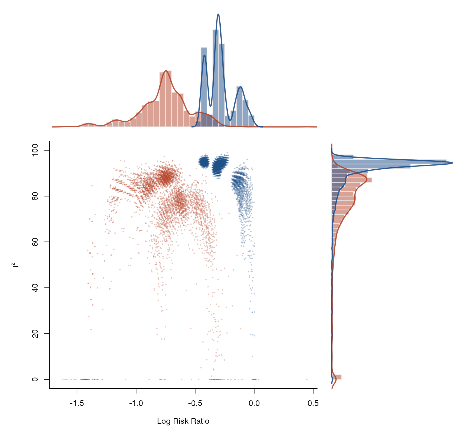
metadat::dat.bcg.
metafor::gosh(), dmetar::gosh.diagnostics()
What it shows
The GOSH plot (Olkin, Dahabreh, and Trikalinos) refits the meta-analysis to every possible subset of the \(k\) studies, or to a large random sample of subsets when \(2^k - 1\) is too many, and plots each subset’s pooled estimate against its heterogeneity. If the studies were homogeneous the cloud would be a single, roughly symmetric blob. Separate clusters mean that the answer depends on which particular studies are included, and coloring subsets by whether they contain a given study shows which study drives the split.
How to read it
- Horizontal axis: pooled estimate of the subset.
- Vertical axis: a heterogeneity statistic, here \(I^2\).
- Each point: one subset of studies.
- Colors: subsets with or without a chosen study.
- Marginal histograms: distributions of the pooled estimate and of \(I^2\).
Interpretation
The cloud splits cleanly by one trial. Subsets containing TPT Madras (blue) form tight clusters with log risk ratios between about −0.45 and 0 and very high \(I^2\), while subsets without it (red) spread from about −1.6 to −0.2. Heterogeneity is high almost everywhere: 97% of subsets have \(I^2\) above 50%. The large null trial is therefore the main reason the pooled effect is attenuated.
Pitfalls
- The number of subsets grows exponentially; for more than about 15 studies use random subsets and report how many.
- Clusters are exploratory. Detecting them by eye, or with clustering algorithms, invites over-interpretation.
- Subsets of one or two studies have undefined or degenerate heterogeneity and pile up at \(I^2 = 0\).
Code
library(metafor)

data(dat.bcg, package = "metadat")
dat <- escalc(measure = "RR", ai = tpos, bi = tneg, ci = cpos, di = cneg,
              data = dat.bcg, slab = paste(author, year))

fit <- rma(yi, vi, data = dat, method = "EE")

# Fit the model to all 2^13 - 1 = 8191 subsets of studies
sav <- gosh(fit)

# Highlight subsets that contain the TPT Madras trial (study 8)
plot(sav, out = 8, col = c("#1d4e89", "#b5452b"),
     breaks = 60, cex = 0.4, alpha = 0.3)
References
- Olkin I, Dahabreh IJ, Trikalinos TA. GOSH: a graphical display of study heterogeneity. Res Synth Methods. 2012;3:214-223. doi:10.1002/jrsm.1053
- Viechtbauer W. GOSH plot. The metafor Package. metafor-project.org