Residual deviance plot
Pointwise residual deviance contributions
MA
NMA
ML-NMR
The posterior residual deviance of every data point, which should be about 1 under good fit.
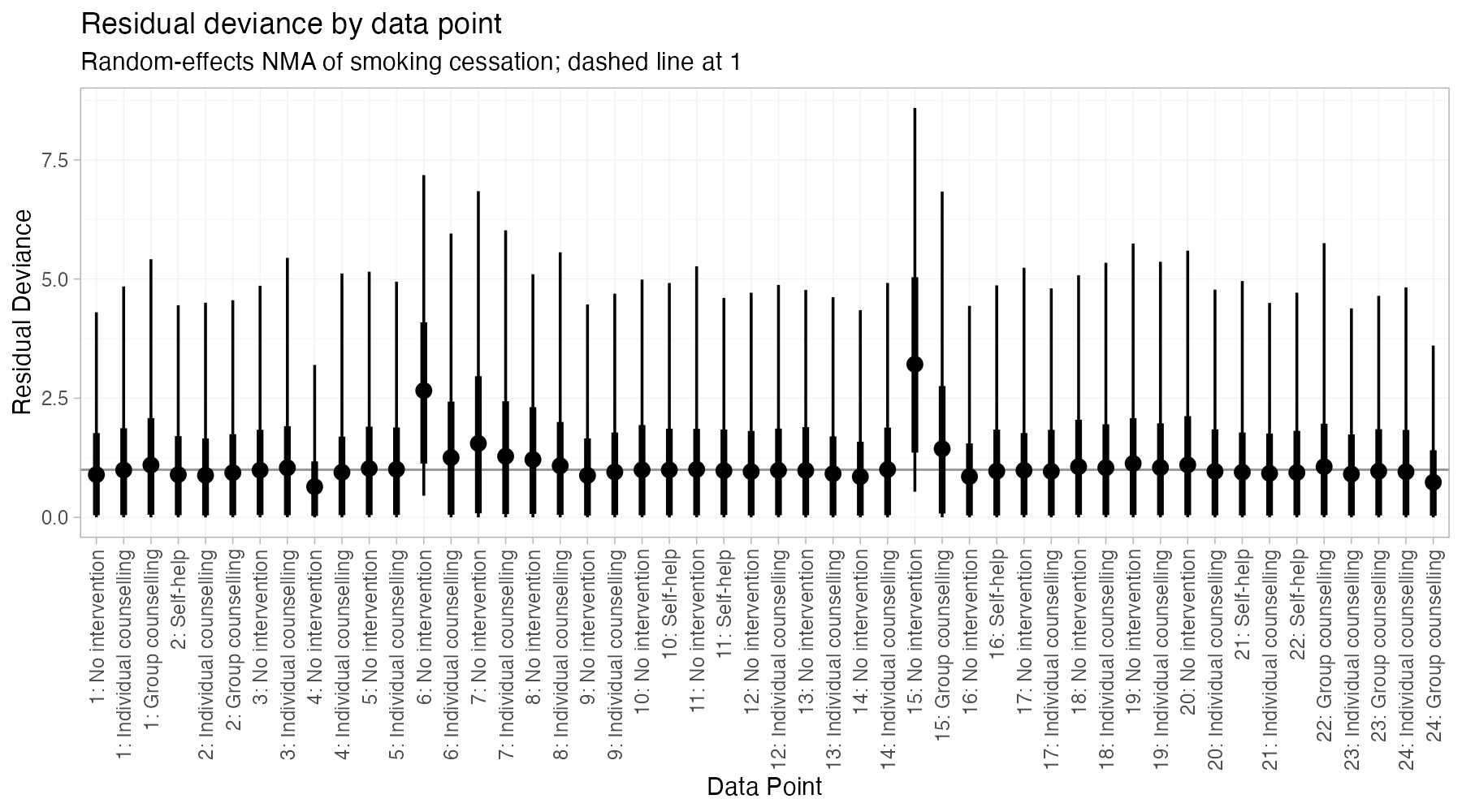
Posterior residual deviance (median and 66% and 95% intervals) for each of the 50 arms in a Bayesian random-effects NMA of 24 smoking cessation trials. Data:
multinma::smoking.
Family
Model checking and Bayesian diagnostics
Purpose
Locate the data points responsible for any lack of fit.
Inputs
Posterior draws of the residual deviance for every data point.
Software
R
multinma::plot(dic()); BUGS or JAGS with custom plots
What it shows
Under a well-fitting model each data point contributes about 1 to the total residual deviance. Plotting the posterior distribution of each point’s contribution, rather than only the total, identifies which arms or studies drive any misfit. It complements the leverage plot and the dev-dev plot.
How to read it
- Horizontal axis: data points, labeled by study and treatment.
- Vertical axis: residual deviance.
- Points and bars: posterior median with 66% and 95% credible intervals.
- Reference: a value of 1 is expected for each point.
Interpretation
Almost all arms sit near 1. The largest contributions come from the no-intervention arms of studies 15 and 6 (posterior means about 3.2 and 2.7), both of which observed zero quitters. Two points with mean deviance near 3 among 50 are not alarming, and the total of 54 for 50 data points indicates adequate fit.
Pitfalls
- Residual deviance for binomial data with zero events has a skewed posterior; do not read the interval as symmetric.
- A few values above 2 or 3 are expected by chance in a large network.
- The plot shows fit, not whether the model’s assumptions (such as consistency) hold.
Code
library(multinma)

net <- set_agd_arm(smoking, study = studyn, trt = trtc, r = r, n = n,
                   trt_ref = "No intervention")

fit <- nma(net, trt_effects = "random",
           prior_intercept = normal(scale = 100),
           prior_trt = normal(scale = 100),
           prior_het = half_normal(scale = 5),
           seed = 2026)

# Posterior residual deviance contribution of every data point (arm);
# each should be about 1 if the model fits
plot(dic(fit)) +
  ggplot2::labs(title = "Residual deviance by data point",
                subtitle = "Random-effects NMA of smoking cessation; dashed line at 1")
References
- Dias S, Welton NJ, Sutton AJ, Ades AE. NICE DSU Technical Support Document 2: A generalised linear modelling framework for pairwise and network meta-analysis of randomised controlled trials. 2011, updated 2016. NCBI Bookshelf NBK310366
- Phillippo DM. multinma: Bayesian network meta-analysis of individual and aggregate data. R package. dmphillippo.github.io/multinma