Influence diagnostics panel
Case-deletion diagnostics, outlier and influence plots
metadat::dat.bcg.
metafor::influence(), metafor::plot.infl.rma.uni()
What it shows
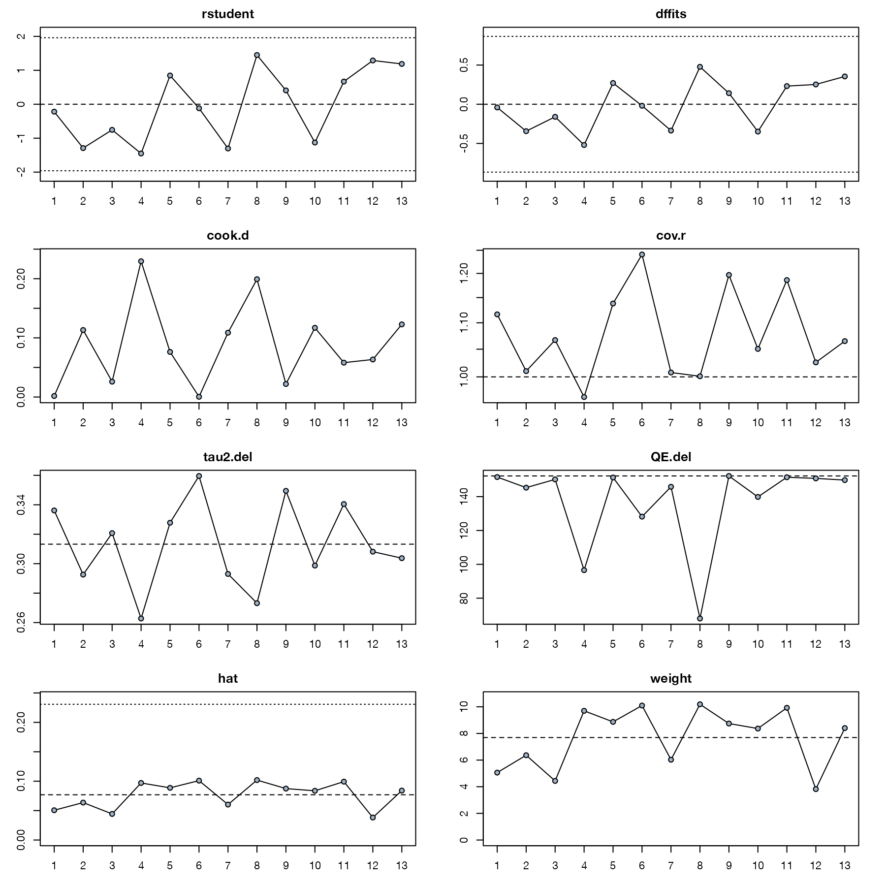
Viechtbauer and Cheung adapted regression case-deletion diagnostics to random-effects meta-analysis. For each study the model is refitted without it and several statistics are computed: externally studentized residuals (outlyingness), DFFITS and Cook’s distance (change in fitted values), covariance ratios (change in precision), the leave-one-out \(\tau^2\) and \(Q\), hat values (leverage), and weights. The panel shows all of them by study index, with reference lines.
How to read it
- Horizontal axis in each panel: study index.
- rstudent: values beyond about ±2 suggest outliers.
- dffits and cook.d: large values mean removing the study changes the fit.
- cov.r: values below 1 mean the study reduces precision when included.
- tau2.del and QE.del: heterogeneity after deleting the study; big drops identify heterogeneity drivers.
- hat and weight: leverage and weight of each study.
- Highlighted points: studies meeting the default influence criteria.
Interpretation
No trial is flagged. Study 4 (Hart and Sutherland) and study 8 (TPT Madras) have the largest Cook’s distances and the largest drops in \(\tau^2\) and \(Q\) when deleted, which matches the Baujat plot. Under the random-effects model, their pull is absorbed by the large between-study variance.
Pitfalls
- Cutoffs are rules of thumb borrowed from regression, not significance tests.
- Diagnostics depend on the model; a study can be influential under a common-effect model and not under random effects.
- With few studies every study is somewhat influential.
- The panel identifies studies to examine for errors or clinical differences; it does not justify excluding them.
Code
library(metafor)

data(dat.bcg, package = "metadat")
dat <- escalc(measure = "RR", ai = tpos, bi = tneg, ci = cpos, di = cneg,
              data = dat.bcg, slab = paste(author, year))

fit <- rma(yi, vi, data = dat, method = "REML")

# Eight case-deletion diagnostics per study; red points flag influential cases
inf <- influence(fit)
plot(inf, bg = "#9fb3c8", bg.infl = "#b5452b", col = "#1d4e89")
References
- Viechtbauer W, Cheung MWL. Outlier and influence diagnostics for meta-analysis. Res Synth Methods. 2010;1:112-125. doi:10.1002/jrsm.11