Prognostic factor curve
Treatment-specific outcome curves across a covariate
mlumr::psoriasis_ipd, psoriasis_agd.
mlumr::conditional_predict() with ggplot2 (shown)
What it shows
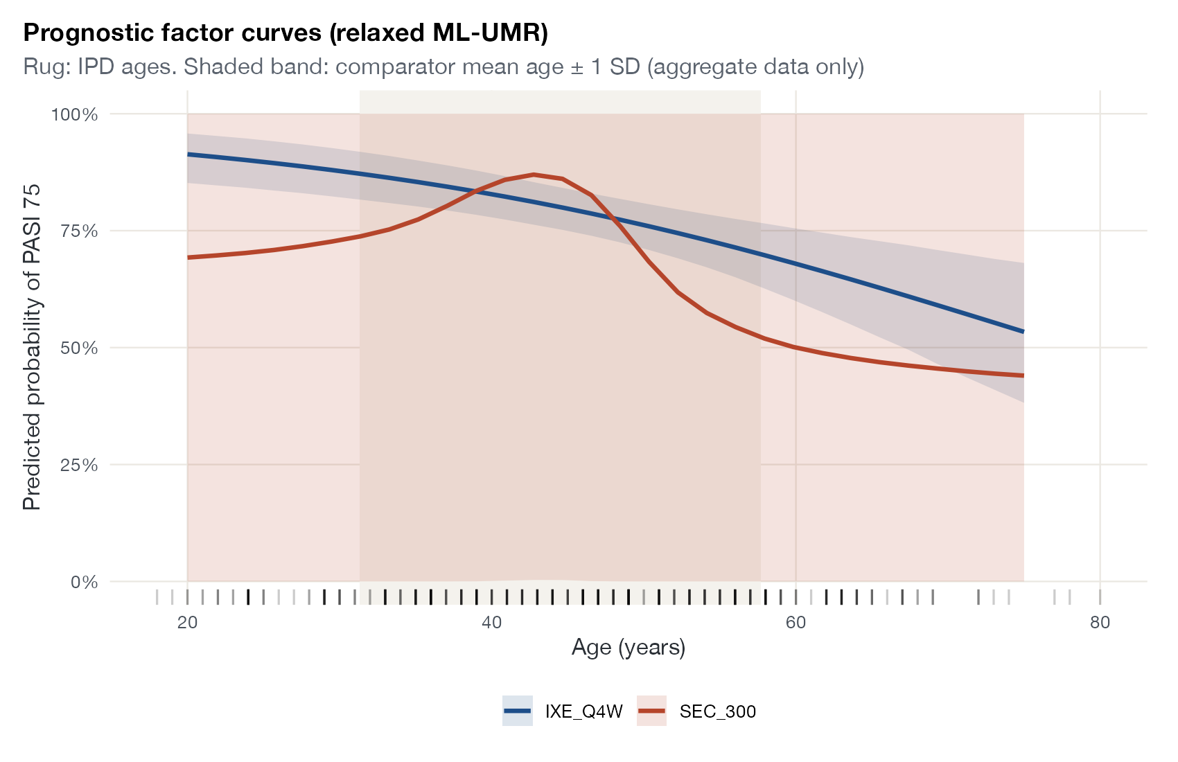
In an unanchored comparison each treatment’s outcome must be modeled as a function of prognostic factors. When covariate effects are allowed to differ by treatment (the relaxed version of the shared prognostic factor assumption), the comparator’s curve has to be learned from aggregate data alone. Plotting both curves across a key covariate, with the IPD distribution and the comparator’s summary marked, shows the strength of each treatment’s evidence at a glance.
How to read it
- Horizontal axis: the prognostic factor.
- Curves and bands: predicted outcome and 95% credible interval for each treatment.
- Rug: covariate values in the IPD.
- Shaded band: the comparator’s covariate mean ± 1 SD.
Interpretation
The ixekizumab curve, estimated from 345 patients, declines smoothly with age and has a narrow band. The secukinumab curve comes from a single aggregate row: near the comparator’s mean age of about 45 it is pinned down by the observed response rate, but away from it the credible band spans almost the entire probability scale. Under the relaxed model the comparator’s age effect is essentially unidentified, which is exactly why ML-UMR offers the stronger shared prognostic factor assumption and why that assumption needs sensitivity analysis.
Pitfalls
- Curves are conditional on the other covariates’ values; state them.
- A narrow band for the IPD treatment says nothing about the comparator’s curve.
- Posterior means of nonlinear functions can look irregular when the posterior is wide; show intervals.
Code
Shared model (R/models/psoriasis-mlumr.R)
# Unanchored comparison of PASI 75 response: ixekizumab Q4W (IPD, UNCOVER-2)
# versus secukinumab 300 mg (aggregate data, FIXTURE), with no common arm
library(mlumr)

ipd <- set_ipd(psoriasis_ipd, treatment = "treatment", outcome = "pasi75",
               covariates = c("age", "bsa", "weight", "prevsys"), family = "binomial")
agd <- set_agd(psoriasis_agd, treatment = "treatment", family = "binomial",
               outcome_n = "pasi75_n", outcome_r = "pasi75_r",
               cov_means = c("age_mean", "bsa_mean", "weight_mean", "prevsys_prop"),
               cov_sds = c("age_sd", "bsa_sd", "weight_sd", NA),
               cov_types = c("continuous", "continuous", "continuous", "binary"))
pso_dat <- combine_data(ipd, agd)

# Integration points over the comparator population's covariate distribution
pso_dat <- add_integration(pso_dat, n_int = 256,
  age = distr(qgamma, mean = age_mean, sd = age_sd),
  bsa = distr(qgamma, mean = bsa_mean, sd = bsa_sd),
  weight = distr(qgamma, mean = weight_mean, sd = weight_sd),
  prevsys = distr(qbern, prob = prevsys_mean))

# Shared prognostic factor model (SPFA) and relaxed model with
# treatment-specific covariate effects
fit_spfa <- mlumr(pso_dat, model = "spfa", seed = 2026, refresh = 0)
fit_relaxed <- mlumr(pso_dat, model = "relaxed", seed = 2026, refresh = 0)
Figure
library(mlumr)
library(ggplot2)
source("R/models/psoriasis-mlumr.R")  # builds pso_dat and fits fit_spfa, fit_relaxed

# Predicted response on each treatment across age, other covariates held at
# the IPD means, from the relaxed model (treatment-specific coefficients)
m <- colMeans(pso_dat$ipd$data[, c("bsa", "weight", "prevsys")])
grid <- data.frame(age = seq(20, 75, length.out = 30), bsa = m[["bsa"]],
                   weight = m[["weight"]], prevsys = m[["prevsys"]])
cp <- conditional_predict(fit_relaxed, newdata = grid)
cp$age <- grid$age[cp$profile]

comp <- psoriasis_agd
ggplot(cp, aes(age, mean, colour = treatment, fill = treatment)) +
  annotate("rect", xmin = comp$age_mean - comp$age_sd, xmax = comp$age_mean + comp$age_sd,
           ymin = -Inf, ymax = Inf, fill = "#f4f2ed") +
  geom_ribbon(aes(ymin = q2.5, ymax = q97.5), alpha = 0.15, colour = NA) +
  geom_line(linewidth = 1.1) +
  geom_rug(data = pso_dat$ipd$data, aes(x = age), inherit.aes = FALSE,
           alpha = 0.2, sides = "b") +
  scale_colour_manual(values = c("#1d4e89", "#b5452b"), name = NULL) +
  scale_fill_manual(values = c("#1d4e89", "#b5452b"), name = NULL) +
  scale_y_continuous(labels = scales::percent) +
  labs(x = "Age (years)", y = "Predicted probability of PASI 75",
       title = "Prognostic factor curves (relaxed ML-UMR)",
       subtitle = "Rug: IPD ages. Shaded band: comparator mean age ± 1 SD (aggregate data only)")
References
- Chandler C, et al. Anchors away: navigating unanchored indirect comparisons with multilevel unanchored meta-regression. 2026. arXiv:2606.20341
- mlumr: Bayesian multilevel unanchored meta-regression. R package. cran.r-project.org/package=mlumr