Leave-one-out forest plot
Sensitivity forest plot, influence analysis forest
MA
NMA
The pooled estimate recomputed after omitting each study in turn, with the resulting heterogeneity.
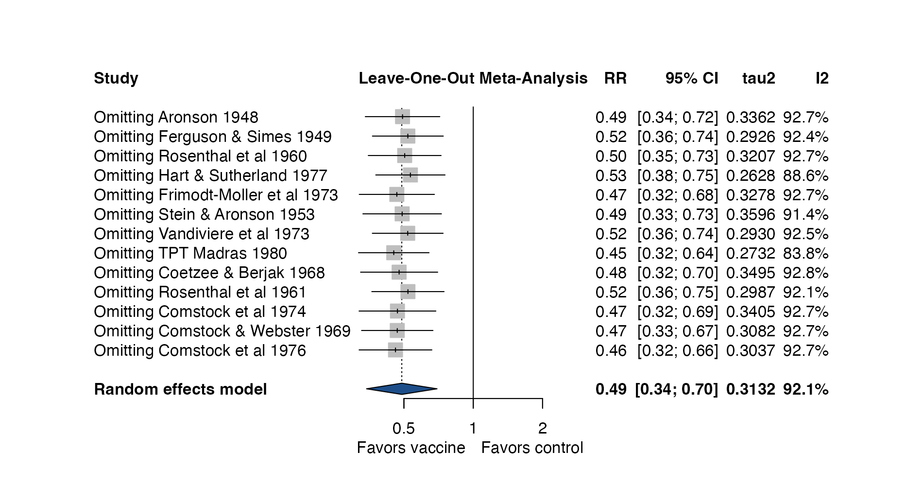
Leave-one-out random-effects meta-analysis of the BCG trials. Each row is the pooled risk ratio with that study removed; the right columns give the corresponding tau² and I². Data:
metadat::dat.bcg.
Family
Heterogeneity and influence
Purpose
Check whether any single study changes the conclusion.
Inputs
Study estimates with standard errors.
Software
R
meta::metainf(), metafor::leave1out(); Stata meta forestplot, leaveoneout
What it shows
Each row of a leave-one-out forest plot is a complete meta-analysis with one study removed. Large shifts in the estimate, interval, or heterogeneity after dropping a study show that the result leans on that study. This is more informative than looking at weights alone, because influence depends on both the weight of a study and how far its result lies from the others.
How to read it
- Rows: labeled by the omitted study.
- Squares and whiskers: pooled estimate and 95% CI without that study.
- Bottom diamond: the full analysis for reference.
- Heterogeneity columns: \(\tau^2\) and \(I^2\) without that study.
Interpretation
The pooled risk ratio stays between 0.45 and 0.53 whatever trial is dropped, and every interval excludes 1, so no single trial carries the conclusion. Omitting TPT Madras gives the largest drop in heterogeneity (\(I^2\) from 92% to 84%) and the strongest effect, consistent with the Baujat plot.
Pitfalls
- A study that changes the result is not thereby wrong; the plot identifies what to investigate, not what to delete.
- Removing studies one at a time cannot reveal influence shared by a group of similar studies; see the GOSH plot.
- In NMA, leaving out a study can disconnect the network or change which comparisons are informed directly.
Code
library(meta)

data(dat.bcg, package = "metadat")

m <- metabin(
  event.e = tpos, n.e = tpos + tneg,
  event.c = cpos, n.c = cpos + cneg,
  studlab = paste(author, year),
  data = dat.bcg, sm = "RR",
  common = FALSE, random = TRUE, method.tau = "REML"
)

# Pooled result after omitting each study in turn
inf <- metainf(m, pooled = "random")

forest(
  inf,
  rightcols = c("effect", "ci", "tau2", "I2"),
  rightlabs = c("RR", "95% CI", "tau2", "I2"),
  label.left = "Favors vaccine", label.right = "Favors control",
  col.square = "#1d4e89", col.diamond = "#1d4e89"
)
meta esize tpos tneg cpos cneg, esize(lnrratio) random(reml)
meta forestplot, eform leaveoneoutReferences
- Viechtbauer W, Cheung MWL. Outlier and influence diagnostics for meta-analysis. Res Synth Methods. 2010;1:112-125. doi:10.1002/jrsm.11
- Balduzzi S, Rücker G, Schwarzer G. How to perform a meta-analysis with R: a practical tutorial. Evid Based Ment Health. 2019;22:153-160. doi:10.1136/ebmental-2019-300117