Effect-modifier curve

Conditional treatment effect across a covariate

The conditional treatment effect against a covariate for each treatment, with the observed IPD and aggregate covariate values marked.

ML-NMRSTCNMIML-UMREstablished

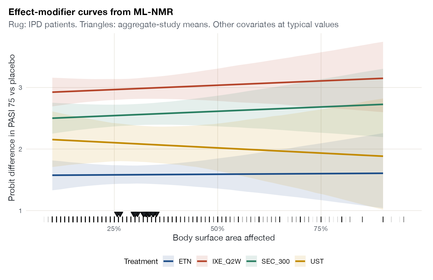
Conditional probit differences in PASI 75 against placebo across body surface area affected, from ML-NMR of the plaque psoriasis network, with other covariates at typical values. Rug: IPD patients; triangles: aggregate-study means. Data: multinma plaque psoriasis example.

Family

Multilevel network meta-regression

Purpose

Show how the treatment effect varies with an effect modifier and where the data support it.

Inputs

A fitted regression model with treatment-covariate interactions.

Software

R multinma::relative_effects(newdata = ) with ggplot2 (shown); emmeans

What it shows

Meta-regression, STC, ML-NMR, NMI, and ML-UMR all imply a relationship between effect modifiers and the treatment effect. Plotting the conditional effect of each treatment against a covariate, with uncertainty bands, makes that relationship explicit. Marking where the IPD lie and where the aggregate studies’ means fall shows whether a target population’s covariate values are within the supported range.

How to read it

• Horizontal axis: the effect modifier.
• Lines and bands: conditional treatment effect and 95% credible interval for each treatment against the reference.
• Rug: IPD covariate values; triangles: aggregate-study means.
• Slope: strength of effect modification.

Interpretation

On the probit scale the lines are nearly flat: body surface area modifies the effect of these biologics only weakly, and the credible bands comfortably include a constant effect. The ordering of treatments (ixekizumab Q2W highest, then secukinumab 300 mg, ustekinumab, and etanercept) holds across the whole range. All aggregate-study means lie between 25% and 35%, well inside the IPD range.

Pitfalls

• Curves are conditional on the other covariates; with interactions, effects at other covariate values differ.
• On nonlinear scales (probit, logit), flat conditional effects can still imply different marginal effects across populations.
• Extrapolating beyond the IPD range relies on the linearity of the interaction.

Code

R

Shared model (R/models/plaque-psoriasis-mlnmr.R)

# ML-NMR of PASI 75 response in plaque psoriasis (Phillippo et al. 2020):
# IPD from 4 ixekizumab trials, aggregate data from 5 secukinumab trials.
library(multinma)
library(dplyr)

trt_class <- function(trtc) case_when(
  trtc == "PBO" ~ "Placebo",
  trtc %in% c("IXE_Q2W", "IXE_Q4W", "SEC_150", "SEC_300") ~ "IL-17 blocker",
  trtc == "ETN" ~ "TNFa blocker",
  trtc == "UST" ~ "IL-12/23 blocker"
)

# Rescale covariates: BSA as a proportion, weight in 10 kg, duration in decades
pso_ipd <- plaque_psoriasis_ipd |>
  mutate(bsa = bsa / 100, weight = weight / 10, durnpso = durnpso / 10,
         prevsys = as.numeric(prevsys), psa = as.numeric(psa),
         trtclass = trt_class(trtc)) |>
  filter(complete.cases(durnpso, prevsys, bsa, weight, psa, pasi75))
pso_agd <- plaque_psoriasis_agd |>
  mutate(bsa_mean = bsa_mean / 100, bsa_sd = bsa_sd / 100,
         weight_mean = weight_mean / 10, weight_sd = weight_sd / 10,
         durnpso_mean = durnpso_mean / 10, durnpso_sd = durnpso_sd / 10,
         prevsys = prevsys / 100, psa = psa / 100,
         trtclass = trt_class(trtc))

pso_net <- combine_network(
  set_ipd(pso_ipd, study = studyc, trt = trtc, r = pasi75, trt_class = trtclass),
  set_agd_arm(pso_agd, study = studyc, trt = trtc, r = pasi75_r, n = pasi75_n,
              trt_class = trtclass),
  trt_ref = "PBO"
)

# Quasi-Monte Carlo integration points over each aggregate study's covariates
pso_net <- add_integration(pso_net,
  durnpso = distr(qgamma, mean = durnpso_mean, sd = durnpso_sd),
  prevsys = distr(qbern, prob = prevsys),
  bsa = distr(qlogitnorm, mean = bsa_mean, sd = bsa_sd),
  weight = distr(qgamma, mean = weight_mean, sd = weight_sd),
  psa = distr(qbern, prob = psa),
  n_int = 64
)

# Fixed-effect ML-NMR, probit link, effect modifiers shared within treatment class
pso_fit <- nma(pso_net, trt_effects = "fixed", link = "probit", likelihood = "bernoulli2",
               regression = ~ (durnpso + prevsys + bsa + weight + psa) * .trt,
               class_interactions = "common",
               prior_intercept = normal(scale = 10), prior_trt = normal(scale = 10),
               prior_reg = normal(scale = 10), init_r = 0.1, QR = TRUE, seed = 2026,
               int_thin = 8, int_check = FALSE)  # save partial integrals for the error plot

Figure

library(multinma)
library(ggplot2)
source("R/models/plaque-psoriasis-mlnmr.R")  # builds pso_net and fits pso_fit

# Conditional probit differences against placebo across body surface area,
# with other covariates held at typical values
grid <- data.frame(bsa = seq(0.1, 0.9, length.out = 40), durnpso = 1.8, prevsys = 0.6,
                   weight = 9, psa = 0.2)
grid$profile <- seq_len(nrow(grid))
re <- as.data.frame(relative_effects(pso_fit, newdata = grid, study = profile))
re$bsa <- grid$bsa[match(re$.study, grid$profile)]
re <- subset(re, .trtb %in% c("ETN", "IXE_Q2W", "SEC_300", "UST"))

obs <- data.frame(bsa = pso_net$ipd$bsa)
agd <- unique(pso_net$agd_arm[, c(".study", "bsa_mean")])

ggplot(re, aes(bsa, mean, colour = .trtb, fill = .trtb)) +
  geom_ribbon(aes(ymin = `2.5%`, ymax = `97.5%`), alpha = 0.12, colour = NA) +
  geom_line(linewidth = 1.1) +
  geom_rug(data = obs, aes(x = bsa), inherit.aes = FALSE, alpha = 0.08, sides = "b") +
  geom_point(data = agd, aes(x = bsa_mean, y = 0.95), inherit.aes = FALSE,
             shape = 25, fill = "#1b1f24", size = 2.4) +
  scale_x_continuous(labels = scales::percent) +
  labs(x = "Body surface area affected", y = "Probit difference in PASI 75 vs placebo",
       colour = "Treatment", fill = "Treatment",
       title = "Effect-modifier curves from ML-NMR",
       subtitle = "Rug: IPD patients. Triangles: aggregate-study means. Other covariates at typical values")

References

• Phillippo DM, Dias S, Ades AE, et al. Multilevel network meta-regression for population-adjusted treatment comparisons. J R Stat Soc Ser A. 2020;183:1189-1210. doi:10.1111/rssa.12579
• Phillippo DM. multinma: Bayesian network meta-analysis of individual and aggregate data. R package. dmphillippo.github.io/multinma