Assumption sensitivity plot
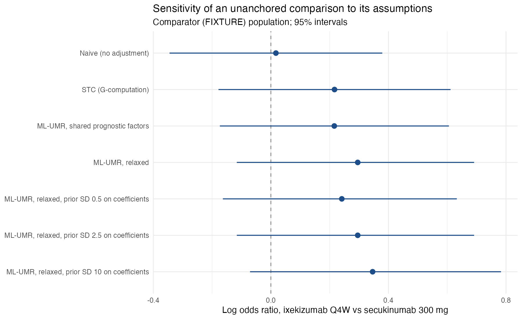
Sensitivity forest for unanchored comparisons, tornado-style display
mlumr::psoriasis_ipd, psoriasis_agd.
mlumr::prior_sensitivity(), mlumr::mlumr_forest() (shown); custom ggplot2 for tornado plots
What it shows
Unanchored comparisons rest on assumptions that the data cannot verify: that all prognostic factors are measured and correctly modeled, and in ML-UMR, whether prognostic effects are shared between treatments (SPFA) or allowed to differ. The NICE DSU describes unanchored population-adjusted comparisons as requiring much stronger assumptions than anchored ones. A sensitivity display lays the same comparison out under each set of choices, so that readers see how much of the conclusion depends on them. A tornado variant lists assumptions on the vertical axis and the resulting change in effect horizontally.
How to read it
- Rows: analyses, ordered from least to most flexible.
- Points and bars: estimate and 95% interval.
- Dashed line: no difference.
- Spread of the points: dependence of the result on assumptions.
Interpretation
The naive comparison finds no difference (log OR 0.02). Adjusting for age, body surface area, weight, and prior systemic therapy, by STC or ML-UMR under SPFA, moves the estimate to about 0.22. Relaxing SPFA gives 0.29, and as the prior on the comparator’s coefficients widens from SD 0.5 to 10 the estimate rises from 0.24 to 0.34 and its interval widens. All intervals include zero, so no analysis supports a difference, but the point estimate depends visibly on untestable modeling choices.
Pitfalls
- A sensitivity plot shows dependence on the assumptions varied, not on those left fixed (for example, unmeasured prognostic factors).
- Choose the grid of assumptions before seeing results.
- Estimands must match across rows: here all rows target the comparator population.
Code
Shared model (R/models/psoriasis-mlumr.R)
# Unanchored comparison of PASI 75 response: ixekizumab Q4W (IPD, UNCOVER-2)
# versus secukinumab 300 mg (aggregate data, FIXTURE), with no common arm
library(mlumr)

ipd <- set_ipd(psoriasis_ipd, treatment = "treatment", outcome = "pasi75",
               covariates = c("age", "bsa", "weight", "prevsys"), family = "binomial")
agd <- set_agd(psoriasis_agd, treatment = "treatment", family = "binomial",
               outcome_n = "pasi75_n", outcome_r = "pasi75_r",
               cov_means = c("age_mean", "bsa_mean", "weight_mean", "prevsys_prop"),
               cov_sds = c("age_sd", "bsa_sd", "weight_sd", NA),
               cov_types = c("continuous", "continuous", "continuous", "binary"))
pso_dat <- combine_data(ipd, agd)

# Integration points over the comparator population's covariate distribution
pso_dat <- add_integration(pso_dat, n_int = 256,
  age = distr(qgamma, mean = age_mean, sd = age_sd),
  bsa = distr(qgamma, mean = bsa_mean, sd = bsa_sd),
  weight = distr(qgamma, mean = weight_mean, sd = weight_sd),
  prevsys = distr(qbern, prob = prevsys_mean))

# Shared prognostic factor model (SPFA) and relaxed model with
# treatment-specific covariate effects
fit_spfa <- mlumr(pso_dat, model = "spfa", seed = 2026, refresh = 0)
fit_relaxed <- mlumr(pso_dat, model = "relaxed", seed = 2026, refresh = 0)
Figure
library(mlumr)
source("R/models/psoriasis-mlumr.R")  # builds pso_dat and fits fit_spfa, fit_relaxed

# The same unanchored log odds ratio under increasingly flexible assumptions,
# in the comparator population
lor <- function(fit) {
  me <- marginal_effects(fit, population = "comparator", effect = "lor")
  c(est = me$mean, lo = me$q2.5, hi = me$q97.5)
}
nv <- naive(pso_dat)
st <- stc(pso_dat, n_boot = 500, seed = 2026)
ps <- prior_sensitivity(fit_relaxed, prior_beta_scales = c(0.5, 2.5, 10), verbose = FALSE)
ps <- subset(ps, parameter == "lor_comparator")
res <- rbind(
  data.frame(label = "Naive (no adjustment)", est = nv$estimate, lo = nv$ci_lower, hi = nv$ci_upper),
  data.frame(label = "STC (G-computation)", est = st$estimate, lo = st$ci_lower, hi = st$ci_upper),
  data.frame(label = "ML-UMR, shared prognostic factors", t(lor(fit_spfa))),
  data.frame(label = "ML-UMR, relaxed", t(lor(fit_relaxed))),
  data.frame(label = paste0("ML-UMR, relaxed, prior SD ", ps$scale, " on coefficients"),
             est = ps$mean, lo = ps$q2.5, hi = ps$q97.5)
)
mlumr_forest(res, ref_line = 0, x = "Log odds ratio, ixekizumab Q4W vs secukinumab 300 mg",
             title = "Sensitivity of an unanchored comparison to its assumptions",
             subtitle = "Comparator (FIXTURE) population; 95% intervals", color = "#1d4e89")
References
- Chandler C, et al. Anchors away: navigating unanchored indirect comparisons with multilevel unanchored meta-regression. 2026. arXiv:2606.20341
- Phillippo DM, Dias S, Ades AE, Welton NJ. Assessing the performance of population adjustment methods for anchored indirect comparisons: a simulation study. Stat Med. 2020;39:4885-4911. doi:10.1002/sim.8759
- Phillippo DM, Ades AE, Dias S, Palmer S, Abrams KR, Welton NJ. NICE DSU Technical Support Document 18: Methods for population-adjusted indirect comparisons in submissions to NICE. 2016. sheffield.ac.uk/nice-dsu