Marginal effect by target population
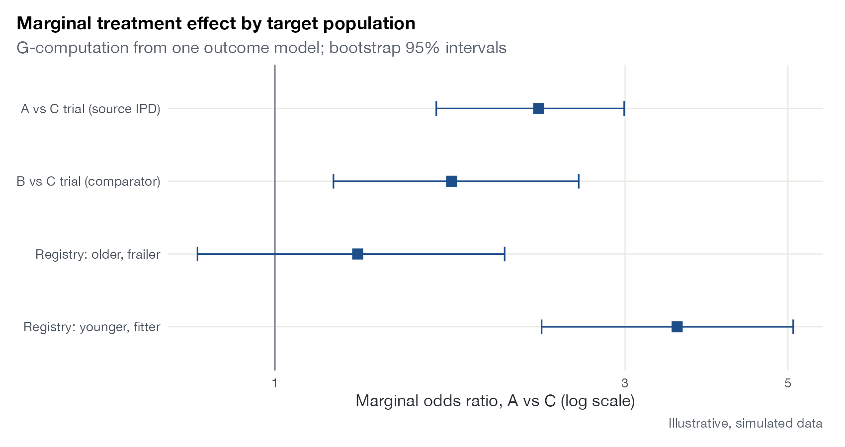
Transportability forest plot, population-specific marginal effects
multinma::marginal_effects(), mlumr::marginal_effects(), stdReg
What it shows
When effect modifiers are present there is no single treatment effect, only effects in particular populations. G-computation (and the marginalization built into ML-NMR and ML-UMR) predicts outcomes under each treatment for everyone in a specified population and contrasts the averages. Displaying the resulting marginal effects for several target populations as rows of a forest plot makes the estimand explicit: which population the decision is about.
How to read it
- Rows: target populations, each defined by a covariate distribution.
- Points and whiskers: marginal effect and its interval in that population.
- Reference line: no effect.
Interpretation
The same outcome model implies a marginal odds ratio of about 2.5 in the trial population, 1.9 in the comparator trial’s older population, 1.3 with an interval crossing 1 in an older, frailer registry population, and about 3.4 in a younger, fitter one. Reporting only one of these without naming its population would mislead any decision about the others.
Pitfalls
- Target covariate distributions built from published means and SDs are assumptions; correlations between covariates must also be assumed.
- The model must include all effect modifiers; otherwise every row inherits the same bias.
- Marginal and conditional effects differ on non-collapsible scales even without effect modification; see the conditional versus marginal plot.
Code
library(ggplot2)

# Simulated IPD from an A vs C trial, with age and ECOG modifying the effect
set.seed(42)
n <- 800
ipd <- data.frame(age = rnorm(n, 60, 9), ecog0 = rbinom(n, 1, 0.45),
                  trt = rep(0:1, each = n / 2))
ipd$y <- rbinom(n, 1, with(ipd, plogis(-1 + 0.04 * (age - 60) + 0.5 * ecog0 +
                                         trt * (0.9 - 0.05 * (age - 60) + 0.4 * ecog0))))
fit <- glm(y ~ trt * (age + ecog0), family = binomial, data = ipd)

# G-computation: predict both treatments for everyone in a simulated target
# population drawn from its published moments, then contrast the averages
marginal_logor <- function(model, mean_age, sd_age, p_ecog0, n = 20000) {
  pop <- data.frame(age = rnorm(n, mean_age, sd_age), ecog0 = rbinom(n, 1, p_ecog0))
  p1 <- mean(predict(model, transform(pop, trt = 1), type = "response"))
  p0 <- mean(predict(model, transform(pop, trt = 0), type = "response"))
  qlogis(p1) - qlogis(p0)
}
targets <- data.frame(
  population = c("A vs C trial (source IPD)", "B vs C trial (comparator)",
                 "Registry: older, frailer", "Registry: younger, fitter"),
  mean_age = c(60, 66, 72, 52), sd_age = c(9, 7, 8, 8), p_ecog0 = c(0.45, 0.35, 0.20, 0.70)
)
res <- do.call(rbind, lapply(seq_len(nrow(targets)), function(i) {
  t <- targets[i, ]
  boots <- replicate(200, {
    b <- ipd[sample(nrow(ipd), replace = TRUE), ]
    marginal_logor(update(fit, data = b), t$mean_age, t$sd_age, t$p_ecog0, n = 4000)
  })
  data.frame(population = t$population, est = marginal_logor(fit, t$mean_age, t$sd_age, t$p_ecog0),
             lo = quantile(boots, 0.025), hi = quantile(boots, 0.975))
}))
res$population <- factor(res$population, levels = rev(targets$population))

ggplot(res, aes(exp(est), population)) +
  geom_vline(xintercept = 1, colour = "#7a828c") +
  geom_errorbar(aes(xmin = exp(lo), xmax = exp(hi)), width = 0.2, orientation = "y",
                colour = "#1d4e89") +
  geom_point(shape = 15, size = 3.4, colour = "#1d4e89") +
  scale_x_log10() +
  labs(x = "Marginal odds ratio, A vs C (log scale)", y = NULL,
       title = "Marginal treatment effect by target population",
       subtitle = "G-computation from one outcome model; bootstrap 95% intervals",
       caption = "Illustrative, simulated data")
References
- Remiro-Azócar A, Heath A, Baio G. Parametric G-computation for compatible indirect treatment comparisons with limited individual patient data. Res Synth Methods. 2022;13:716-744. doi:10.1002/jrsm.1565
- Phillippo DM, Dias S, Ades AE, et al. Multilevel network meta-regression for population-adjusted treatment comparisons. J R Stat Soc Ser A. 2020;183:1189-1210. doi:10.1111/rssa.12579