Prior versus posterior plot

Prior-posterior overlay

NMA

ML-NMR

ML-UMR

Prior densities overlaid on posterior distributions, showing how much the data updated each parameter.

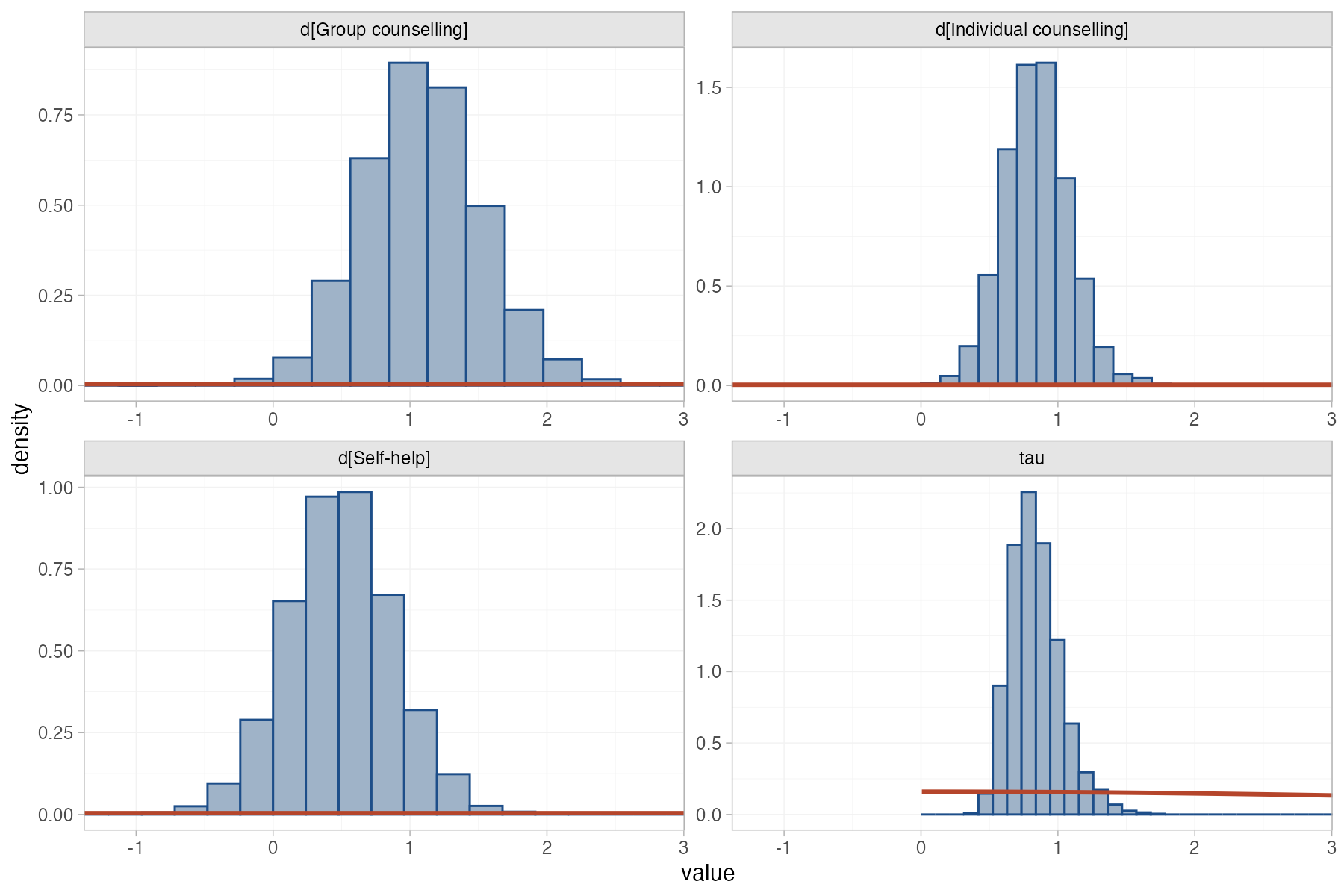
Posterior distributions (histograms) and prior densities (red lines) of the treatment effects (log odds ratios versus no intervention) and heterogeneity SD in a Bayesian random-effects NMA of smoking cessation. Priors are normal(0, 100²) for effects and half-normal(0, 5²) for tau. Data: multinma::smoking.

Family

Model checking and Bayesian diagnostics

Purpose

Show whether results are driven by the data or by the priors.

Inputs

Prior specifications and posterior draws.

Software

R multinma::plot_prior_posterior(), bayesmeta::plot(prior = TRUE), bayesplot

What it shows

Overlaying each parameter’s prior on its posterior shows at a glance how much the data informed it. When the posterior is much narrower than the prior, the data dominate. When the two nearly coincide, the parameter is weakly identified and the result reflects the prior. This matters most for the heterogeneity parameter in sparse networks, for treatment-by-covariate interactions in ML-NMR, and for the prognostic-factor parameters that carry unanchored ML-UMR comparisons.

How to read it

Histogram: posterior draws.
Line: prior density on the same scale.
Panels: one per parameter.

Interpretation

Both priors are essentially flat over the region where the posterior lies, so every parameter is informed by the data. The posterior for \(\tau\) is centered near 0.82 (95% CrI 0.54 to 1.28), well inside a prior that would have allowed values up to about 10. With vague priors like these the plot confirms that choice of prior is not driving the result.

Pitfalls

A vague prior can still be informative on a transformed scale, or when data are sparse (for example a flat prior on log odds implies a U-shaped prior on probability).
Agreement between prior and posterior is not a problem if the prior was deliberately informative; it becomes one when it was supposed to be vague.
Pair the plot with a formal prior sensitivity analysis for key parameters.

Code

library(multinma)

net <- set_agd_arm(smoking, study = studyn, trt = trtc, r = r, n = n,
                   trt_ref = "No intervention")

fit <- nma(net, trt_effects = "random",
           prior_intercept = normal(scale = 100),
           prior_trt = normal(scale = 100),
           prior_het = half_normal(scale = 5),
           seed = 2026)

# Prior (line) and posterior (histogram) for the heterogeneity SD tau and
# the treatment effects: how much did the data update each prior?
plot_prior_posterior(fit, prior = c("trt", "het"),
                     post_args = list(fill = "#9fb3c8", colour = "#1d4e89"),
                     prior_args = list(colour = "#b5452b", linewidth = 1))

References

Röver C, Bender R, Dias S, et al. On weakly informative prior distributions for the heterogeneity parameter in Bayesian random-effects meta-analysis. Res Synth Methods. 2021;12:448-474. doi:10.1002/jrsm.1475
Phillippo DM. multinma: Bayesian network meta-analysis of individual and aggregate data. R package. dmphillippo.github.io/multinma