Transitivity plot

Effect-modifier distribution plot, covariate balance across comparisons

NMA

ML-NMR

NMI

ITC

The distribution of potential effect modifiers across trials or direct comparisons, to judge whether indirect comparisons are plausible.

NMA ML-NMR NMI ITCEstablished

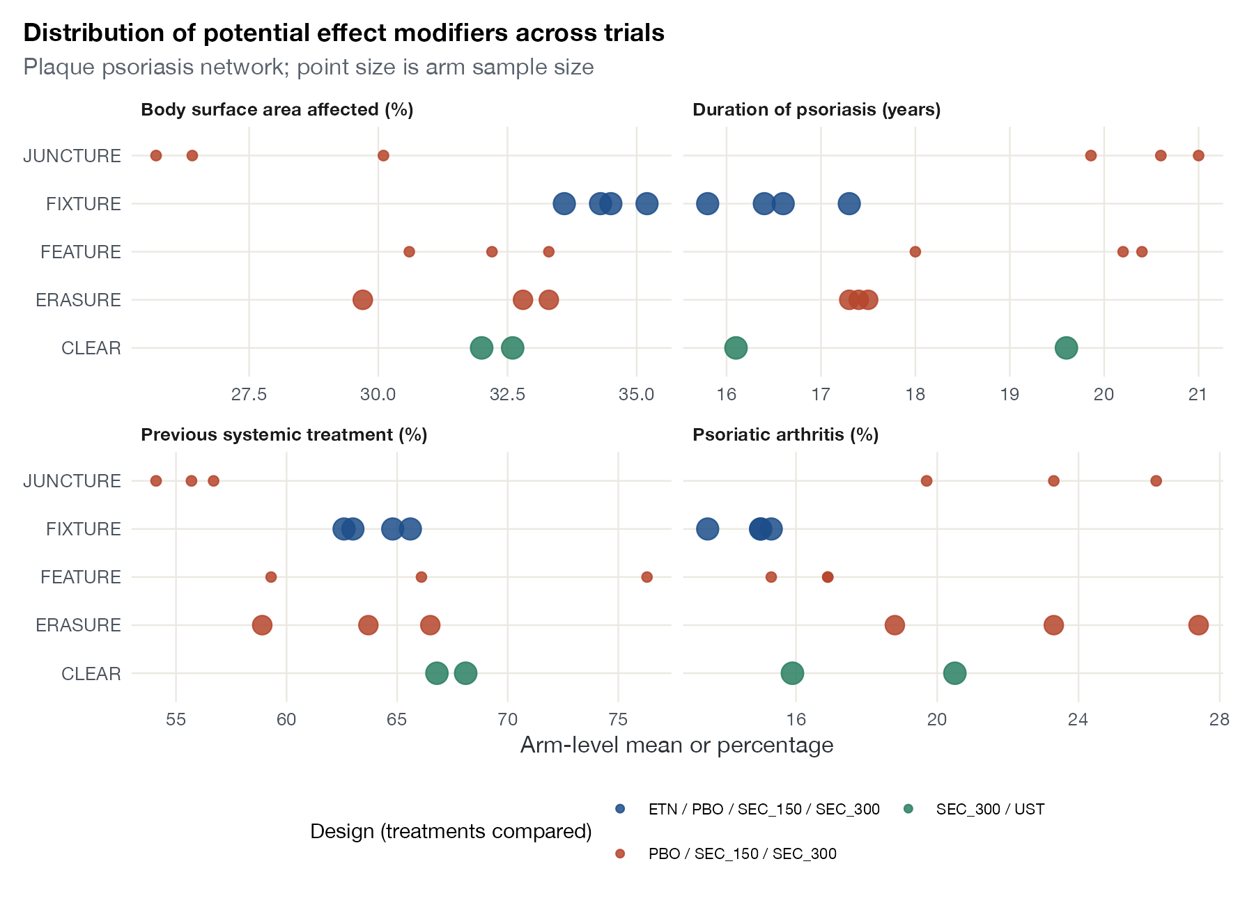
Arm-level means or percentages of four potential effect modifiers in the five trials of the plaque psoriasis network, colored by trial design. Point size reflects arm sample size. Data: multinma::plaque_psoriasis_agd.

Family

Network geometry and evidence flow

Purpose

Assess the transitivity (similarity) assumption before trusting indirect comparisons.

Inputs

Study- or arm-level summaries of effect modifiers; IPD where available.

Software

R ggplot2; Stata network summaries; multinma data

What it shows

Indirect comparisons and network meta-analysis are valid only if effect modifiers are similarly distributed across the comparisons being combined. The transitivity plot puts the evidence for that assumption on the page: for each important patient or study characteristic, it shows the value in every trial (or arm), grouped by the treatments compared. Imbalance across designs is exactly the situation that motivates network meta-regression, ML-NMR, and NMI.

How to read it

Panels: one per potential effect modifier, chosen on clinical grounds.
Rows: trials; colors: design (set of treatments compared).
Points: arm-level means or percentages; size reflects sample size.
Look for: systematic differences in a covariate between designs, not scatter within a design.

Interpretation

The JUNCTURE and FEATURE trials (placebo and secukinumab only) enrolled patients with longer disease duration (about 20 years against 16 to 17 in FIXTURE) and smaller affected body surface area. Previous systemic treatment ranges from about 54% in JUNCTURE to 76% in one FEATURE arm. If disease duration or prior treatment modifies the response to biologics, indirect comparisons through placebo mix different populations, which is the motivation for the ML-NMR analysis of these data.

Pitfalls

Only covariates that are reported can be compared; unreported effect modifiers remain unchecked.
Means and percentages hide differences in distribution. Do not draw full distributions reconstructed from means and SDs without labeling them as assumptions.
The plot cannot tell which covariates are effect modifiers; that needs clinical knowledge or evidence from within trials.

Code

library(multinma)
library(ggplot2)

# Plaque psoriasis: aggregate baseline characteristics of 5 trials (per arm)
agd <- plaque_psoriasis_agd
agd$design <- ave(agd$trtc, agd$studyc, FUN = function(t) paste(sort(unique(t)), collapse = " / "))

long <- rbind(
  data.frame(study = agd$studyc, design = agd$design, n = agd$sample_size_w0,
             covariate = "Duration of psoriasis (years)", value = agd$durnpso_mean),
  data.frame(study = agd$studyc, design = agd$design, n = agd$sample_size_w0,
             covariate = "Previous systemic treatment (%)", value = agd$prevsys),
  data.frame(study = agd$studyc, design = agd$design, n = agd$sample_size_w0,
             covariate = "Body surface area affected (%)", value = agd$bsa_mean),
  data.frame(study = agd$studyc, design = agd$design, n = agd$sample_size_w0,
             covariate = "Psoriatic arthritis (%)", value = agd$psa)
)

# Potential effect modifiers by trial design: one point per arm
ggplot(long, aes(x = value, y = study, colour = design)) +
  geom_point(aes(size = n), alpha = 0.85) +
  facet_wrap(~ covariate, scales = "free_x", ncol = 2) +
  scale_size_area(max_size = 5, guide = "none") +
  labs(x = "Arm-level mean or percentage", y = NULL, colour = "Design (treatments compared)",
       title = "Distribution of potential effect modifiers across trials",
       subtitle = "Plaque psoriasis network; point size is arm sample size") +
  guides(colour = guide_legend(ncol = 2)) +
  theme(legend.text = element_text(size = 8))

References

Salanti G. Indirect and mixed-treatment comparison, network, or multiple-treatments meta-analysis: many names, many benefits, many concerns for the next generation evidence synthesis tool. Res Synth Methods. 2012;3:80-97. doi:10.1002/jrsm.1037
Cipriani A, Higgins JPT, Geddes JR, Salanti G. Conceptual and technical challenges in network meta-analysis. Ann Intern Med. 2013;159:130-137. doi:10.7326/0003-4819-159-2-201307160-00008
Phillippo DM, Dias S, Ades AE, et al. Multilevel network meta-regression for population-adjusted treatment comparisons. J R Stat Soc Ser A. 2020;183:1189-1210. doi:10.1111/rssa.12579