Conditional versus marginal effect plot
Non-collapsibility plot
ggplot2 (shown)
What it shows
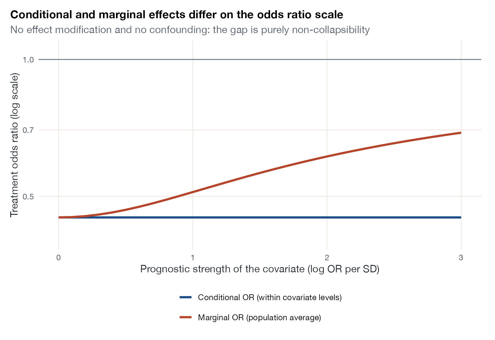
Odds ratios and hazard ratios are non-collapsible: the population-average (marginal) effect differs from the within-stratum (conditional) effect even when the covariate is not an effect modifier and not a confounder. Conventional STC plugs covariate means into a conditional regression and compares the result with a published marginal effect, mixing the two. This proof-of-concept plot, of the kind used in the methodological literature, shows how large the gap can become as a covariate’s prognostic effect grows.
How to read it
- Horizontal axis: strength of the covariate’s prognostic effect.
- Blue line: the conditional odds ratio, constant by construction.
- Red line: the marginal odds ratio in the population.
- Gap between them: the estimand mismatch.
Interpretation
With no prognostic covariate the two coincide at 0.45. As the covariate’s effect grows to 3 log-odds units per SD, the marginal odds ratio attenuates to about 0.69, although nothing about the treatment has changed. An STC that reports the conditional value against a published marginal comparator would overstate the treatment benefit.
Pitfalls
- The gap is not bias in either quantity; each is correct for its own estimand. The error lies in comparing them.
- Risk differences and mean differences on the identity link are collapsible and do not show this pattern.
- G-computation, ML-NMR, and ML-UMR marginalize over the covariate distribution to produce a coherent marginal effect.
Code
library(ggplot2)

# Non-collapsibility of the odds ratio: with the conditional log OR fixed at
# -0.8, the marginal log OR moves toward zero as the prognostic effect of a
# covariate (not an effect modifier) grows
set.seed(1)
x <- rnorm(2e5)
strength <- seq(0, 3, by = 0.1)
marg <- sapply(strength, function(b) {
  p1 <- mean(plogis(-0.5 - 0.8 + b * x))
  p0 <- mean(plogis(-0.5 + b * x))
  qlogis(p1) - qlogis(p0)
})
d <- rbind(data.frame(strength, logor = -0.8, type = "Conditional OR (within covariate levels)"),
           data.frame(strength, logor = marg, type = "Marginal OR (population average)"))

ggplot(d, aes(strength, exp(logor), colour = type)) +
  geom_hline(yintercept = 1, colour = "#7a828c") +
  geom_line(linewidth = 1.2) +
  scale_colour_manual(values = c("#1d4e89", "#b5452b"), name = NULL) +
  scale_y_log10(limits = c(0.4, 1.05)) +
  labs(x = "Prognostic strength of the covariate (log OR per SD)",
       y = "Treatment odds ratio (log scale)",
       title = "Conditional and marginal effects differ on the odds ratio scale",
       subtitle = "No effect modification and no confounding: the gap is purely non-collapsibility") +
  guides(colour = guide_legend(ncol = 1))
References
- Remiro-Azócar A, Heath A, Baio G. Parametric G-computation for compatible indirect treatment comparisons with limited individual patient data. Res Synth Methods. 2022;13:716-744. doi:10.1002/jrsm.1565
- Daniel R, Zhang J, Farewell D. Making apples from oranges: comparing noncollapsible effect estimators and their standard errors after adjustment for different covariate sets. Biom J. 2021;63:528-557. doi:10.1002/bimj.201900297