Anchored indirect comparison diagram
Bucher plot, adjusted indirect comparison forest
maicplus::bucher(), netmeta, custom ggplot2; any spreadsheet
What it shows
When A and B have never been compared head to head but both have been compared with C, the Bucher method estimates A versus B as the difference of the two anchored effects on the linear predictor scale:
\[ \hat d_{AB} = \hat d_{AC} - \hat d_{BC}, \qquad \operatorname{Var}(\hat d_{AB}) = \operatorname{Var}(\hat d_{AC}) + \operatorname{Var}(\hat d_{BC}). \]
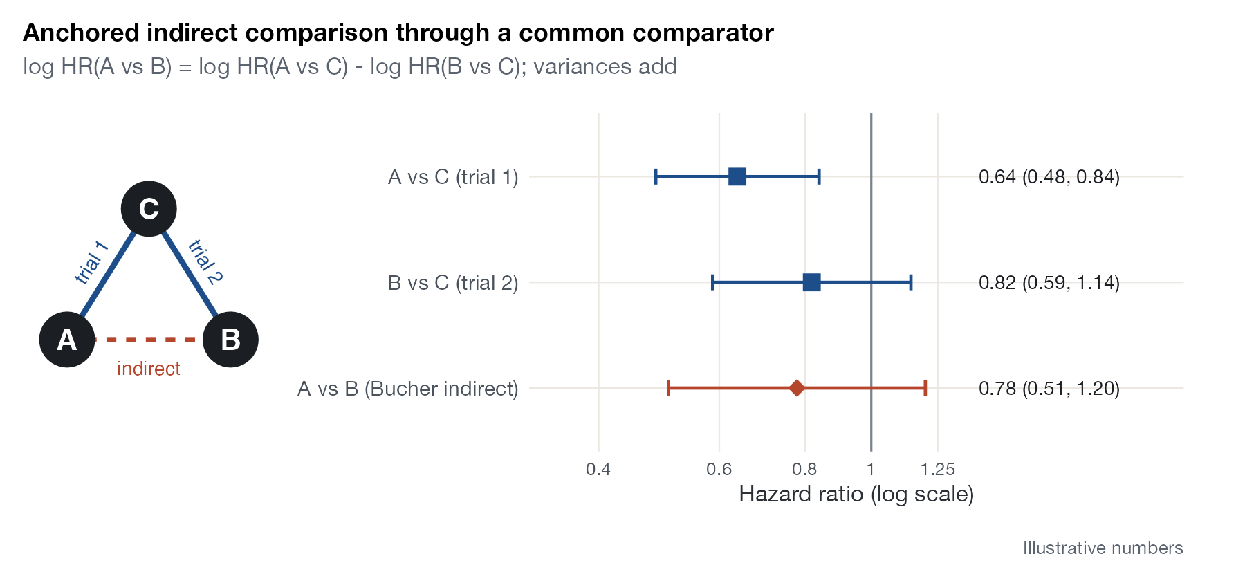
The diagram pairs a small network sketch with a forest plot of the inputs and the result, so that readers see both the evidence structure and the loss of precision. It is the simplest possible network meta-analysis, and the basis against which MAIC and STC are compared.
How to read it
- Network sketch: solid edges are randomized comparisons; the dashed edge is the comparison being inferred.
- Forest rows: the two anchored (direct) estimates and the indirect estimate.
- Interval widths: the indirect interval is always wider than either input, because variances add.
- Right-hand labels: hazard ratios with 95% confidence intervals.
Interpretation
A reduces the hazard relative to C (HR 0.64) and B does so less (HR 0.82), giving an indirect HR for A versus B of 0.78 (95% CI 0.51 to 1.20). Both inputs are fairly precise, yet the indirect interval includes 1: indirect evidence is weaker than direct evidence of the same size.
Pitfalls
- Validity rests on the similarity (transitivity) assumption: effect modifiers must be balanced between the AC and BC trials. The diagram cannot show that; population-adjusted methods such as MAIC exist because it often fails.
- Subtract on the log scale for ratio measures, never on the natural scale.
- The comparator arms must be the same treatment, dose, and background therapy.
- An unanchored comparison (no common comparator) is not a Bucher comparison; it relies on much stronger assumptions.
Code
library(ggplot2)
library(patchwork)

# Two placebo-controlled trials: A vs C and B vs C (log hazard ratios)
ac <- c(est = -0.45, se = 0.14)
bc <- c(est = -0.20, se = 0.17)

# Bucher adjusted indirect comparison: difference of the two anchored effects
ab <- c(est = ac[["est"]] - bc[["est"]], se = sqrt(ac[["se"]]^2 + bc[["se"]]^2))

d <- data.frame(
  row = factor(c("A vs C (trial 1)", "B vs C (trial 2)", "A vs B (Bucher indirect)"),
               levels = rev(c("A vs C (trial 1)", "B vs C (trial 2)", "A vs B (Bucher indirect)"))),
  est = c(ac[["est"]], bc[["est"]], ab[["est"]]),
  se = c(ac[["se"]], bc[["se"]], ab[["se"]]),
  type = c("Direct", "Direct", "Indirect")
)
d$lo <- d$est - 1.96 * d$se
d$hi <- d$est + 1.96 * d$se

forest <- ggplot(d, aes(x = est, y = row, colour = type)) +
  geom_vline(xintercept = 0, colour = "#7a828c") +
  geom_errorbar(aes(xmin = lo, xmax = hi), width = 0.15, orientation = "y", linewidth = 0.8) +
  geom_point(aes(shape = type), size = 4) +
  geom_text(aes(x = 0.36, label = sprintf("%.2f (%.2f, %.2f)", exp(est), exp(lo), exp(hi))),
            colour = "#1b1f24", hjust = 0, size = 3.6) +
  scale_shape_manual(values = c(Direct = 15, Indirect = 18)) +
  scale_colour_manual(values = c(Direct = "#1d4e89", Indirect = "#b5452b")) +
  scale_x_continuous(breaks = log(c(0.4, 0.6, 0.8, 1, 1.25)),
                     labels = c(0.4, 0.6, 0.8, 1, 1.25), limits = c(-1.05, 0.95)) +
  labs(x = "Hazard ratio (log scale)", y = NULL, colour = NULL, shape = NULL) +
  theme(legend.position = "none", axis.text.y = element_text(size = 11))

nodes <- data.frame(x = c(0, 2, 1), y = c(0, 0, 1.6), lab = c("A", "B", "C"))
network <- ggplot() +
  annotate("segment", x = 0, y = 0, xend = 1, yend = 1.6, colour = "#1d4e89", linewidth = 1.4) +
  annotate("segment", x = 2, y = 0, xend = 1, yend = 1.6, colour = "#1d4e89", linewidth = 1.4) +
  annotate("segment", x = 0, y = 0, xend = 2, yend = 0, colour = "#b5452b",
           linewidth = 1.2, linetype = "22") +
  geom_point(data = nodes, aes(x, y), size = 13, colour = "#1b1f24") +
  geom_text(data = nodes, aes(x, y, label = lab), colour = "white", size = 5.5, fontface = "bold") +
  annotate("text", x = 1, y = -0.35, label = "indirect", colour = "#b5452b", size = 3.6) +
  annotate("text", x = 0.3, y = 0.95, label = "trial 1", colour = "#1d4e89", size = 3.6, angle = 58) +
  annotate("text", x = 1.7, y = 0.95, label = "trial 2", colour = "#1d4e89", size = 3.6, angle = -58) +
  coord_equal(xlim = c(-0.4, 2.4), ylim = c(-0.6, 2)) +
  theme_void()

network + forest + plot_layout(widths = c(1, 2.6)) +
  plot_annotation(
    title = "Anchored indirect comparison through a common comparator",
    subtitle = "log HR(A vs B) = log HR(A vs C) - log HR(B vs C); variances add",
    caption = "Illustrative numbers"
  )
References
- Bucher HC, Guyatt GH, Griffith LE, Walter SD. The results of direct and indirect treatment comparisons in meta-analysis of randomized controlled trials. J Clin Epidemiol. 1997;50:683-691. doi:10.1016/S0895-4356(97)00049-8
- Glenny AM, Altman DG, Song F, et al. Indirect comparisons of competing interventions. Health Technol Assess. 2005;9(26). doi:10.3310/hta9260