Forest plot with risk-of-bias columns

RoB-annotated forest plot

A forest plot with a traffic-light column for each risk-of-bias domain beside every study.

MAEstablished

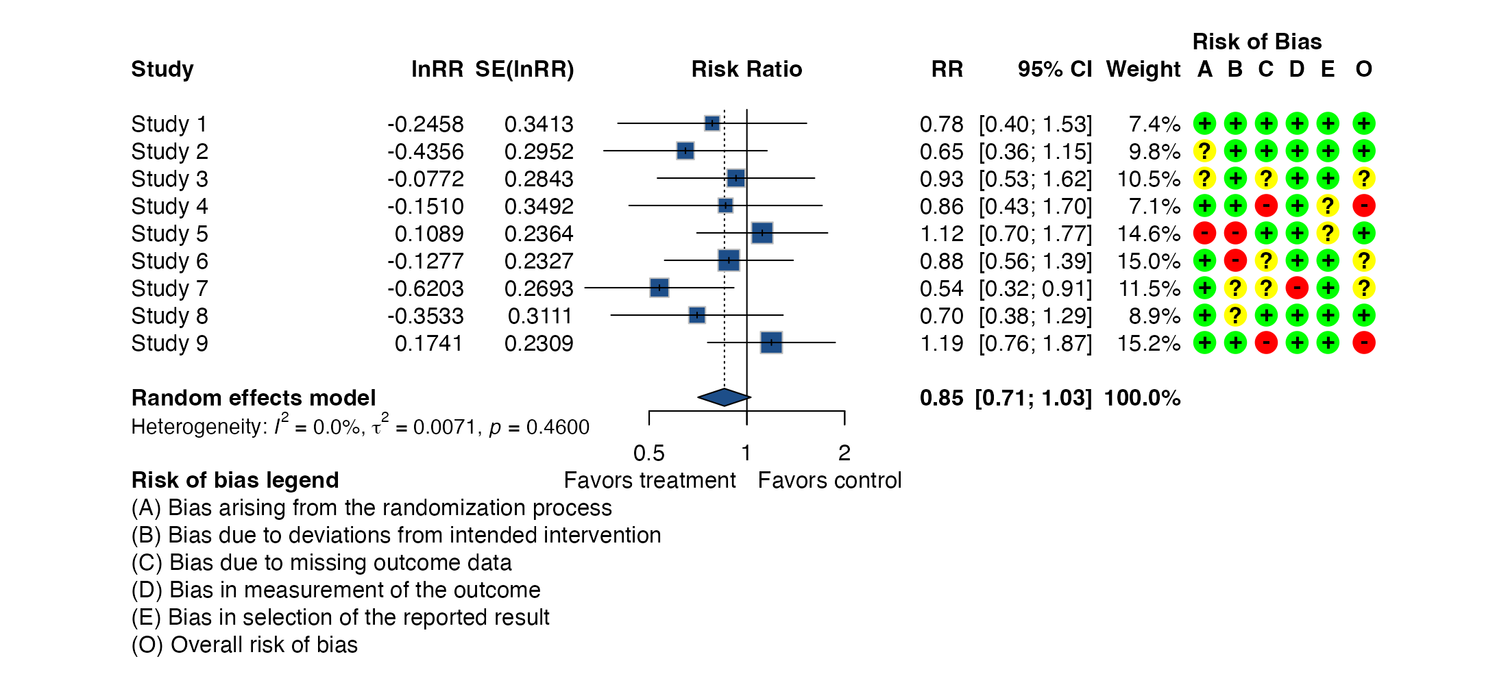
Random-effects meta-analysis of nine example studies with RoB 2 judgments (domains A to E and overall) shown beside each study. Effect estimates are illustrative; judgments are from robvis::data_rob2.

Family

Risk of bias and reporting

Purpose

Show risk of bias next to each study’s result, so readers can see whether biased studies drive the pooled estimate.

Inputs

Study effects and domain-level risk-of-bias judgments.

Software

R meta::rob() + forest(), robvis::rob_append_to_forest(); RevMan

What it shows

Placing risk-of-bias judgments beside each row of a forest plot, as RevMan and recent versions of meta do, lets readers connect bias to results directly: do the high-risk studies show larger effects, and would the conclusion change without them?

How to read it

Left and middle: a standard forest plot.
Right columns: judgment for each domain (A to E) and overall (O), with a legend below.

Interpretation

The pooled risk ratio is 0.85 (95% CI 0.71 to 1.03) with no heterogeneity. The two studies at high overall risk (studies 4 and 9) have estimates close to or above 1, and the largest benefit comes from study 7, which is at high risk for outcome measurement. A sensitivity analysis restricted to low-risk studies would be the natural next step.

Pitfalls

Visual association between bias and effect across a few studies is weak evidence; use subgroup analysis or meta-regression by risk of bias if needed.
Crowded plots with many domains need careful layout.

Code

library(meta)
library(robvis)

# RoB 2 judgments for nine example studies (robvis) paired with
# illustrative effect estimates
data(data_rob2)
set.seed(4)
dat <- data.frame(study = data_rob2$Study,
                  TE = rnorm(9, -0.3, 0.25), seTE = runif(9, 0.12, 0.35))
dat <- cbind(dat, data_rob2[, c("D1", "D2", "D3", "D4", "D5", "Overall")])

m <- metagen(TE, seTE, studlab = study, data = dat, sm = "RR",
             common = FALSE, random = TRUE)

# Attach the risk of bias table; forest() then adds the traffic-light columns
m <- rob(D1, D2, D3, D4, D5, overall = Overall, data = m, tool = "RoB2")
forest(m, col.square = "#1d4e89", col.diamond = "#1d4e89",
       label.left = "Favors treatment", label.right = "Favors control")

References

McGuinness LA, Higgins JPT. Risk-of-bias VISualization (robvis): an R package and Shiny web app for visualizing risk-of-bias assessments. Res Synth Methods. 2021;12:55-61. doi:10.1002/jrsm.1411
Balduzzi S, Rücker G, Schwarzer G. How to perform a meta-analysis with R: a practical tutorial. Evid Based Ment Health. 2019;22:153-160. doi:10.1136/ebmental-2019-300117