Clustered ranking plot
Two-dimensional ranking plot, efficacy versus acceptability scatter
NMA
Ranking scores for two outcomes plotted against each other, with treatments grouped by hierarchical clustering.
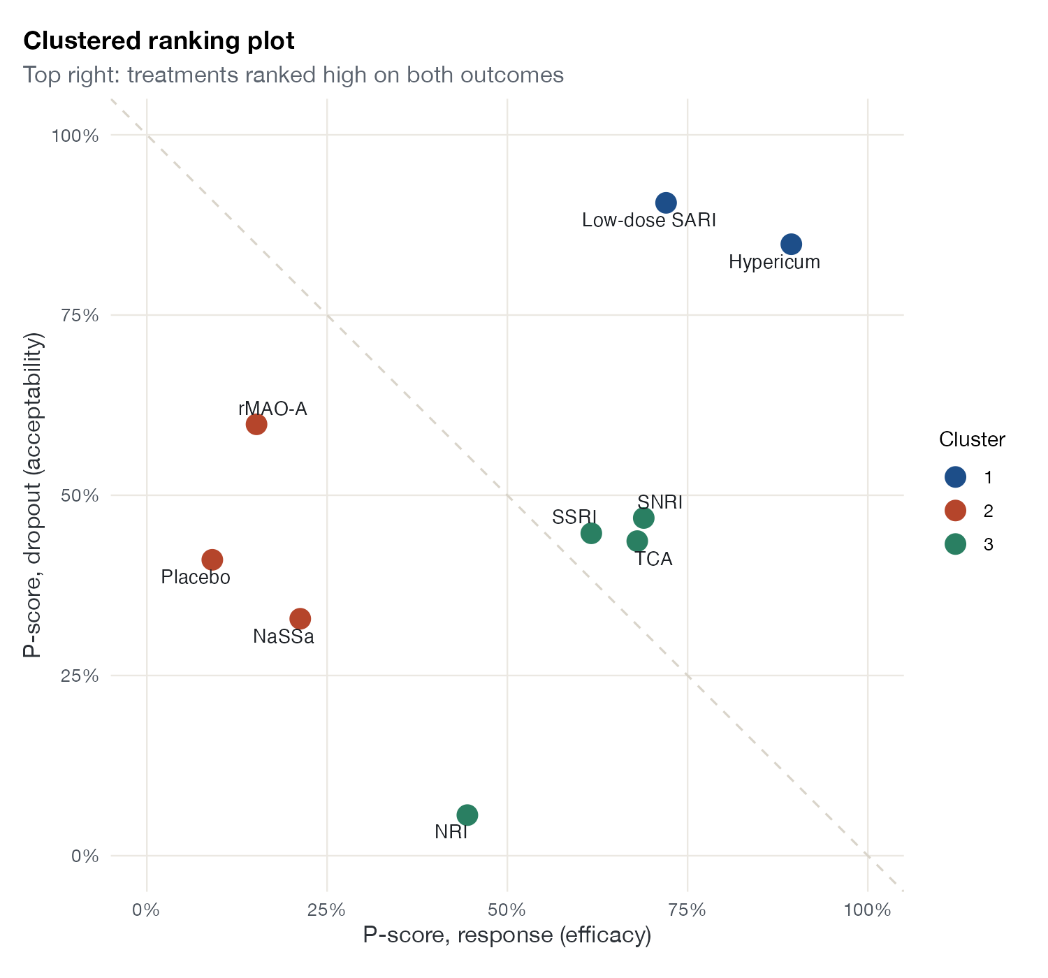
P-scores for response (efficacy) against dropout (acceptability) in the antidepressant network, colored by three clusters from Ward’s hierarchical clustering. Data:
netmeta::Linde2015.
Family
Treatment ranking
Purpose
Identify groups of treatments with similar benefit-harm profiles.
Inputs
Ranking scores for two (or more) outcomes.
Software
Stata
clusterank; R hclust() with ggplot2 (shown)
What it shows
Chaimani and colleagues proposed plotting SUCRA values for two outcomes, usually efficacy and acceptability, against each other and grouping treatments by hierarchical clustering. Treatments in the top right do well on both; clusters summarize the benefit-harm landscape.
How to read it
- Horizontal axis: ranking score for the first outcome (efficacy).
- Vertical axis: ranking score for the second outcome (acceptability).
- Colors: clusters.
- Dashed diagonal: equal sum of the two scores.
Interpretation
Low-dose SARI and hypericum form a cluster in the top right. SSRI, SNRI, and TCA form a middle cluster with good efficacy and average acceptability, and NRI falls into the same cluster despite the worst acceptability. Placebo, NaSSa, and rMAO-A form a low-efficacy cluster.
Pitfalls
- Clusters depend on the distance metric, the linkage method, and the number of clusters, all of which are choices.
- Ranking scores ignore effect sizes; two treatments in the same cluster may still differ importantly.
- Do not present clusters as an objective taxonomy of treatments.
Code
library(netmeta)

# Antidepressants in primary care (Linde et al. 2015): arm-level binary outcomes
data(Linde2015)
d <- Linde2015
nma_for <- function(v, small) {
  p <- pairwise(treat = list(d$treatment1, d$treatment2, d$treatment3),
                event = list(d[[paste0(v, 1)]], d[[paste0(v, 2)]], d[[paste0(v, 3)]]),
                n = list(d$n1, d$n2, d$n3), studlab = d$id, sm = "OR", allstudies = TRUE)
  netmeta(p, common = FALSE, reference.group = "Placebo", small.values = small)
}
library(ggplot2)

resp <- nma_for("resp", small = "undesirable")
loss <- nma_for("loss", small = "desirable")

ps <- data.frame(treatment = resp$trts,
                 efficacy = netrank(resp)$ranking.random[resp$trts],
                 acceptability = netrank(loss)$ranking.random[resp$trts])

# Hierarchical clustering on the two ranking scores (Ward's method)
cl <- hclust(dist(ps[, c("efficacy", "acceptability")]), method = "ward.D2")
ps$group <- factor(cutree(cl, k = 3))

ggplot(ps, aes(efficacy, acceptability, colour = group)) +
  geom_abline(slope = -1, intercept = 1, colour = "#d9d4ca", linetype = "dashed") +
  geom_point(size = 4.5) +
  ggrepel::geom_text_repel(aes(label = treatment), size = 3.5, colour = "#1b1f24",
                           point.padding = 0.5) +
  scale_x_continuous(limits = c(0, 1), labels = scales::percent) +
  scale_y_continuous(limits = c(0, 1), labels = scales::percent) +
  coord_equal() +
  labs(x = "P-score, response (efficacy)", y = "P-score, dropout (acceptability)",
       colour = "Cluster", title = "Clustered ranking plot",
       subtitle = "Top right: treatments ranked high on both outcomes") +
  theme(legend.position = "right")
clusterank sucra_eff sucra_acc, best(max) method(ward)References
- Chaimani A, Higgins JPT, Mavridis D, Spyridonos P, Salanti G. Graphical tools for network meta-analysis in STATA. PLoS One. 2013;8:e76654. doi:10.1371/journal.pone.0076654
- Cipriani A, Furukawa TA, Salanti G, et al. Comparative efficacy and acceptability of 12 new-generation antidepressants: a multiple-treatments meta-analysis. Lancet. 2009;373:746-758. doi:10.1016/S0140-6736(09)60046-5