Copas selection model plot
Copas sensitivity analysis plot
metadat::dat.hackshaw1998.
metasens::copas(), metasens::plot.copas()
What it shows
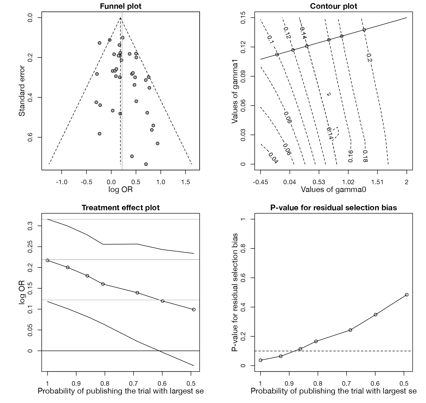
The Copas model links each study’s chance of publication to its precision through two parameters, \(\gamma_0\) and \(\gamma_1\). Because these cannot be estimated from the observed studies alone, the model is used as a sensitivity analysis: the pooled estimate is computed across a grid of selection strengths. The four panels show the data, the grid, the resulting treatment effects, and whether the funnel asymmetry is still unexplained at each level of selection.
How to read it
- Funnel plot: the observed data.
- Contour plot: adjusted estimates across combinations of \(\gamma_0\) and \(\gamma_1\); the solid line is the path used in the lower panels.
- Treatment effect plot: adjusted estimate with confidence limits as the probability of publishing the least precise study decreases from 1 (no selection) to the left of the axis.
- Residual selection bias plot: p-value for the remaining asymmetry; values above the dashed 0.1 line mean the selection model explains the asymmetry.
Interpretation
With no selection the odds ratio is 1.24. At the point where residual asymmetry is no longer significant (about 86% chance of publishing the least precise study, four unpublished studies), the estimate is 1.20 (95% CI 1.09 to 1.32). Only under stronger selection, with the least precise study published about 60% of the time or less, does the interval include 1. The association survives moderate selection.
Pitfalls
- The analysis is a sensitivity analysis over unidentifiable parameters; the “adjusted estimate” depends on the stopping rule.
- The model assumes selection depends on precision in a particular way.
- The contour plot can be unstable when there are few studies.
Code
library(meta)
library(metasens)

data(dat.hackshaw1998, package = "metadat")

m <- metagen(TE = yi, seTE = sqrt(vi), studlab = paste(author, year),
             data = dat.hackshaw1998, sm = "OR")

# Copas selection model: funnel, contour of adjusted estimates over the
# selection parameters, adjusted estimate against probability of publishing
# the smallest study, and p-value for residual selection bias
cop <- copas(m)
plot(cop)
References
- Copas J, Shi JQ. Meta-analysis, funnel plots and sensitivity analysis. Biostatistics. 2000;1:247-262. doi:10.1093/biostatistics/1.3.247
- Carpenter JR, Schwarzer G, Rücker G, Künstler R. Empirical evaluation showed that the Copas selection model provided a useful summary in 80% of meta-analyses. J Clin Epidemiol. 2009;62:624-631. doi:10.1016/j.jclinepi.2008.12.002