Observed versus predicted plot
Calibration plot, observed against fitted
NMA
STC
ML-NMR
ML-UMR
Observed arm-level or study-level outcomes against model predictions, around the line of perfect agreement.
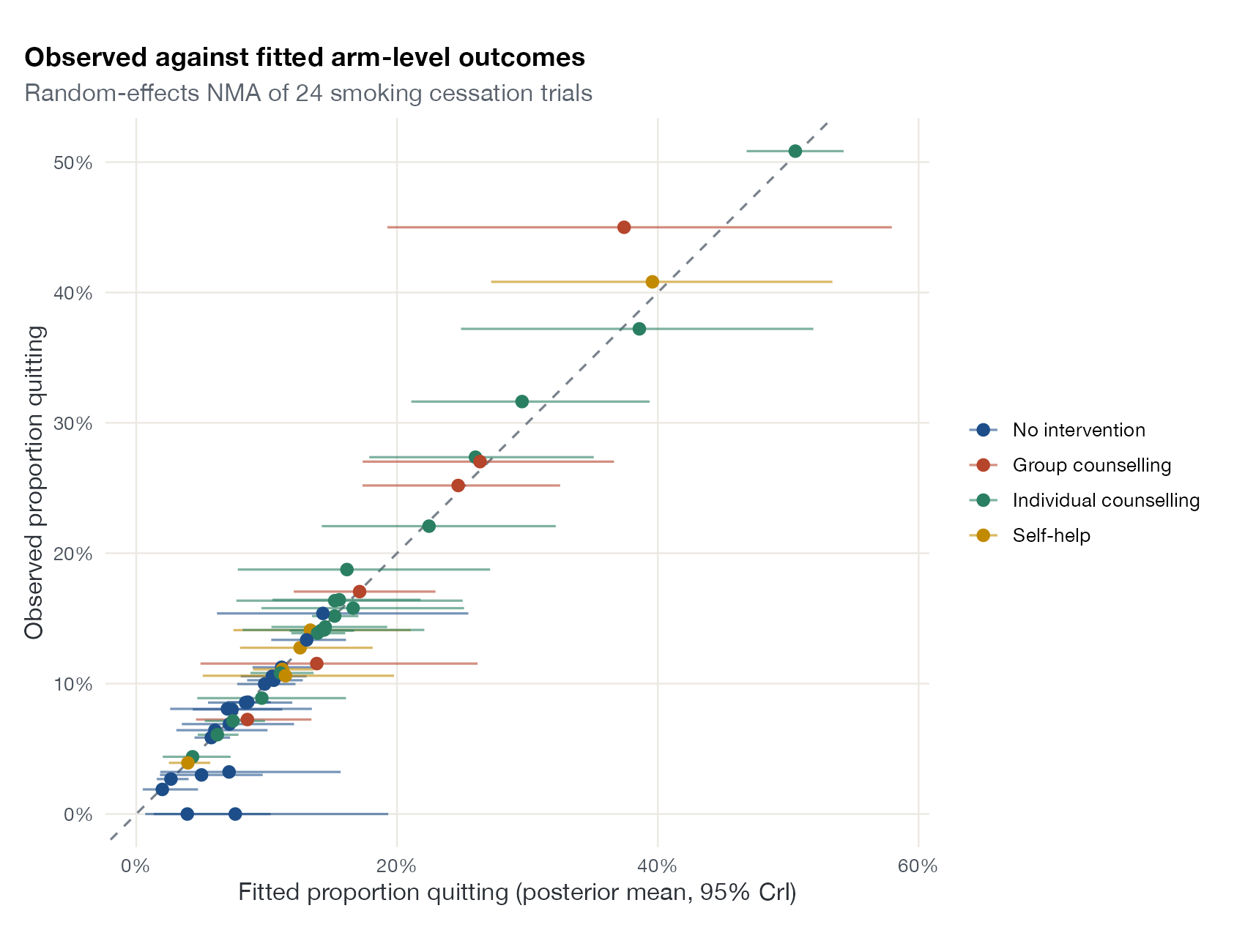
Observed against posterior fitted proportions quitting for all 50 arms of a Bayesian random-effects NMA of smoking cessation, with 95% credible intervals, colored by treatment. Data:
multinma::smoking.
Family
Model checking and Bayesian diagnostics
Purpose
Check whether a model reproduces observed outcomes on their natural scale.
Inputs
Observed outcomes and model-based predictions for the same units.
Software
R
multinma fitted values, ggplot2; any regression software
What it shows
Plotting what was observed against what the model predicts for the same arms, studies, or patient groups is the most direct check of calibration. Points should lie along the 45° line. It is especially useful for outcome-regression methods (STC, G-computation, ML-NMR, ML-UMR), where absolute predictions drive the result, and for arm-based NMA models, where baseline risks are modeled.
How to read it
- Horizontal axis: fitted value (posterior mean with credible interval).
- Vertical axis: observed value.
- Dashed line: perfect agreement.
- Colors: treatment or study group.
Interpretation
Arms fall close to the diagonal across the full range of quit rates, from under 5% to about 50%. Intervals are wide for small arms, and the arms observing zero quitters sit below the line, as expected when a random-effects model shrinks them. There is no systematic departure by treatment.
Pitfalls
- In random-effects models each arm is partly fitted from its own data, so agreement is expected; it is not external validation.
- For STC and G-computation, calibration on the IPD used for fitting says nothing about transportability to the aggregate-data population.
- Aggregate calibration can hide poor fit in covariate subgroups.
Code
library(multinma)
library(ggplot2)

net <- set_agd_arm(smoking, study = studyn, trt = trtc, r = r, n = n,
                   trt_ref = "No intervention")

fit <- nma(net, trt_effects = "random",
           prior_intercept = normal(scale = 100),
           prior_trt = normal(scale = 100),
           prior_het = half_normal(scale = 5),
           seed = 2026)

# Posterior fitted event proportions for each arm against the observed ones
fitted <- as.matrix(fit, pars = "fitted_agd_arm")
arms <- net$agd_arm
d <- data.frame(
  observed = arms$.r / arms$.n,
  fitted = colMeans(fitted) / arms$.n,
  lo = apply(fitted, 2, quantile, 0.025) / arms$.n,
  hi = apply(fitted, 2, quantile, 0.975) / arms$.n,
  treatment = arms$.trt
)

ggplot(d, aes(fitted, observed, colour = treatment)) +
  geom_abline(colour = "#7a828c", linetype = "dashed") +
  geom_errorbar(aes(xmin = lo, xmax = hi), orientation = "y", width = 0, alpha = 0.6) +
  geom_point(size = 2.4) +
  coord_equal() +
  scale_x_continuous(labels = scales::percent) +
  scale_y_continuous(labels = scales::percent) +
  labs(x = "Fitted proportion quitting (posterior mean, 95% CrI)",
       y = "Observed proportion quitting", colour = NULL,
       title = "Observed against fitted arm-level outcomes",
       subtitle = "Random-effects NMA of 24 smoking cessation trials") +
  theme(legend.position = "right")
References
- Dias S, Welton NJ, Sutton AJ, Ades AE. NICE DSU Technical Support Document 2. 2011, updated 2016. NCBI Bookshelf NBK310366
- Phillippo DM, Dias S, Ades AE, et al. Multilevel network meta-regression for population-adjusted treatment comparisons. J R Stat Soc Ser A. 2020;183:1189-1210. doi:10.1111/rssa.12579