Normal Q-Q plot
Quantile-quantile plot of standardized residuals
MA
NMA
Standardized residuals against normal quantiles, with a simulated envelope, to check the normality assumption of the random-effects model.
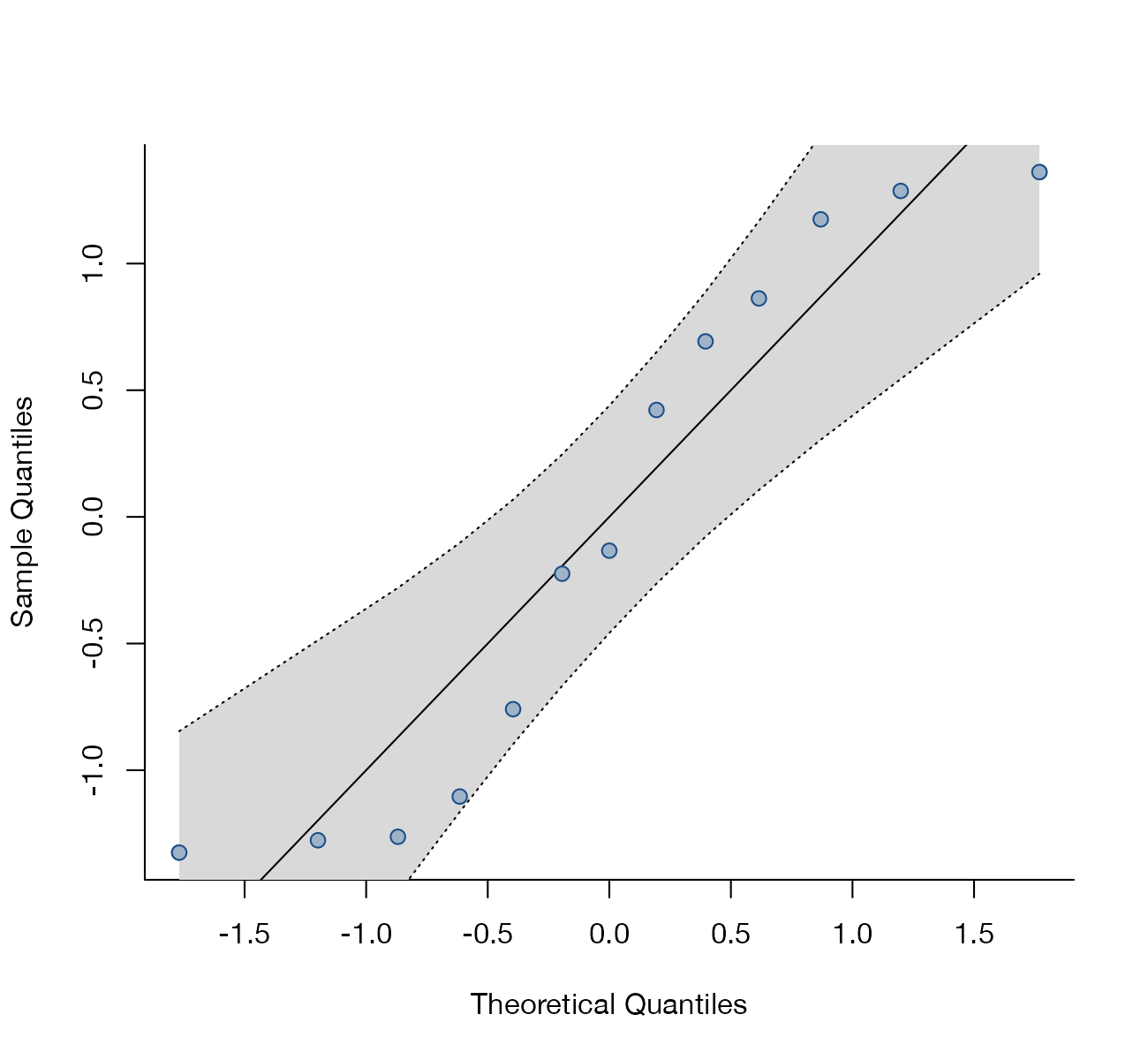
Normal Q-Q plot of standardized residuals from a REML random-effects model of the 13 BCG trials, with a 95% pseudo-confidence envelope from simulation. Data:
metadat::dat.bcg.
Family
Model checking and Bayesian diagnostics
Purpose
Check the normality of residuals or random effects and spot outlying studies.
Inputs
A fitted random-effects model.
Software
R
metafor::qqnorm(), meta; Stata qnorm on residuals
What it shows
Random-effects meta-analysis assumes that true effects are normally distributed around the mean. Plotting ordered standardized residuals against the quantiles expected under normality shows whether that assumption is reasonable. Points should fall along the diagonal. A simulated envelope (Wang and Bushman) shows how much scatter to expect by chance with this number of studies.
How to read it
- Horizontal axis: theoretical normal quantiles.
- Vertical axis: ordered standardized residuals.
- Diagonal line: perfect normality.
- Shaded envelope: 95% pseudo-confidence region from data simulated under the fitted model.
Interpretation
All 13 residuals lie within the envelope, with a mild S shape: the tails are a little shorter than normal. With so few studies there is no reason to reject the normal random-effects assumption, and equally little power to detect a violation.
Pitfalls
- With few studies Q-Q plots have almost no power; the envelope is wide.
- Residuals are not independent after estimation, and empirical Bayes estimates of random effects are shrunk; a Q-Q plot of shrunken estimates understates departures from normality.
- Skewed or bimodal true effects can hide behind a well-behaved Q-Q plot if they are few.
Code
library(metafor)

data(dat.bcg, package = "metadat")
dat <- escalc(measure = "RR", ai = tpos, bi = tneg, ci = cpos, di = cneg,
              data = dat.bcg, slab = paste(author, year))

fit <- rma(yi, vi, data = dat, method = "REML")

# Standardized residuals against normal quantiles, with a simulated
# 95% pseudo-confidence envelope
qqnorm(fit, pch = 21, bg = "#9fb3c8", col = "#1d4e89", envelope = TRUE,
       main = "", label = "out", cex = 1.1)
References
- Wang MC, Bushman BJ. Using the normal quantile plot to explore meta-analytic data sets. Psychol Methods. 1998;3:46-54. doi:10.1037/1082-989X.3.1.46
- Viechtbauer W. Conducting meta-analyses in R with the metafor package. J Stat Softw. 2010;36(3):1-48. doi:10.18637/jss.v036.i03