Bayesian shrinkage forest plot
Forest plot with posterior (shrunken) study estimates
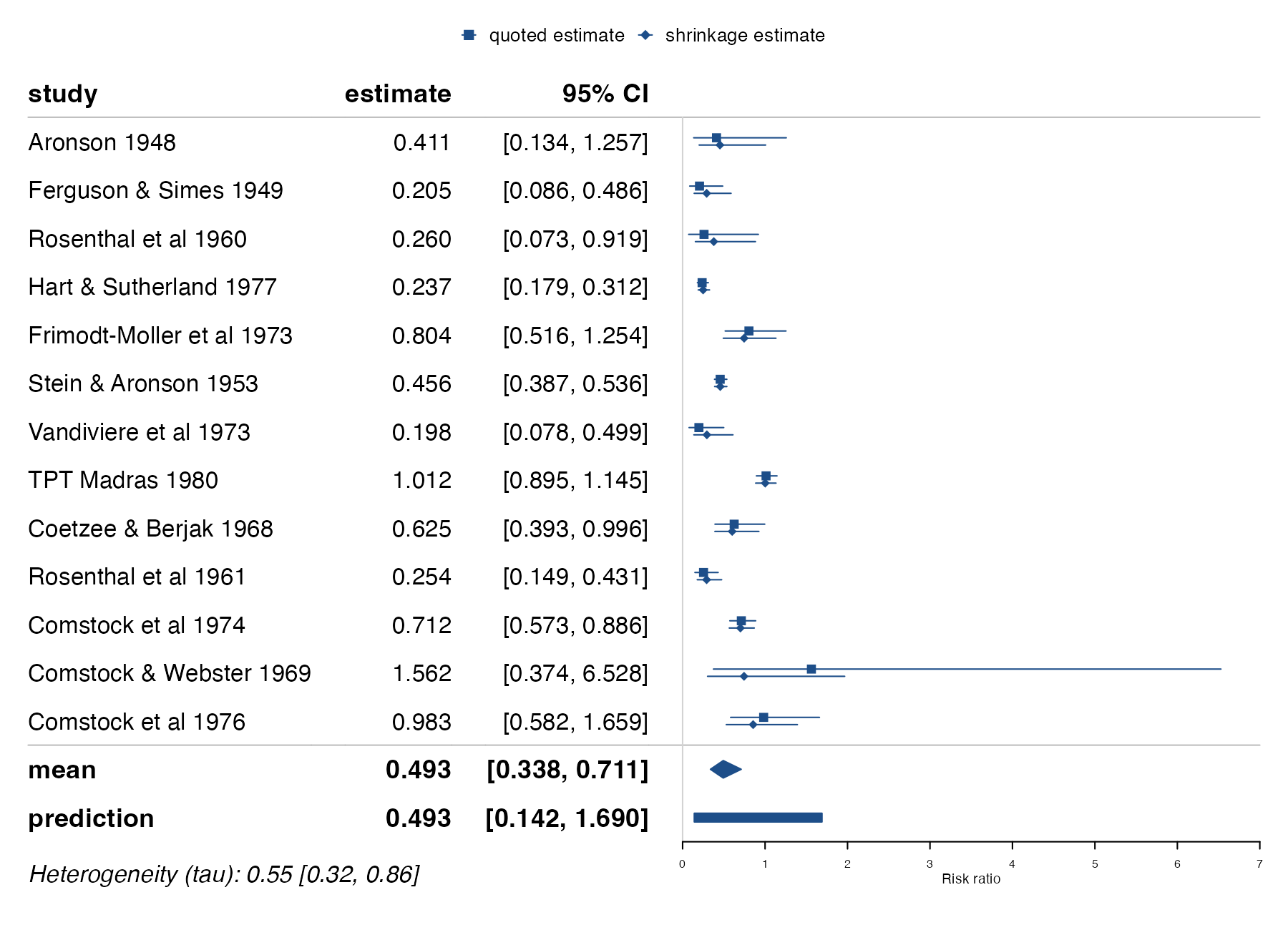
metadat::dat.bcg.
bayesmeta::forestplot(), brms, multinma; Stan or JAGS
What it shows
In a random-effects model each study has its own true effect, drawn from a common distribution. The posterior for each study-specific effect combines that study’s data with what the other studies say about the distribution, so estimates are “shrunk” toward the mean. The shrinkage forest plot draws both versions: the quoted estimate and the shrunken estimate. Imprecise studies move the most; precise studies barely move.
How to read it
- Squares with lines: the quoted estimate and 95% confidence interval of each study.
- Diamonds with lines: the posterior mean and 95% credible interval of each study’s true effect.
- Mean row: posterior of the overall mean effect \(\mu\).
- Prediction row: posterior predictive interval for a new study’s true effect.
- Heterogeneity line: posterior median and interval for \(\tau\).
Interpretation
Comstock and Webster, with only eight events, is shrunk from 1.56 to below 1, while the large TPT Madras trial stays near 1.01. The posterior mean risk ratio is 0.49 (95% CrI 0.34 to 0.71), \(\tau\) is 0.55 (0.32 to 0.86), and the predictive interval runs from 0.14 to 1.69. The shrinkage estimates are the better guess of each setting’s true effect under the exchangeability assumption.
Pitfalls
- Shrinkage is only as sensible as the exchangeability assumption; a study that differs systematically should not be pulled toward the others.
- The amount of shrinkage depends on the prior for \(\tau\), especially with few studies. Report the prior and consider a sensitivity analysis.
- Shrunken estimates are not new data; they reuse the other studies’ results.
Code
library(metafor)
library(bayesmeta)

data(dat.bcg, package = "metadat")
dat <- escalc(measure = "RR", ai = tpos, bi = tneg, ci = cpos, di = cneg,
              data = dat.bcg)

# Bayesian random-effects model with a half-normal prior on tau
bm <- bayesmeta(
  y = dat$yi, sigma = sqrt(dat$vi),
  labels = paste(dat$author, dat$year),
  mu.prior.mean = 0, mu.prior.sd = 4,
  tau.prior = function(t) dhalfnormal(t, scale = 0.5)
)

# Gray lines: shrinkage (posterior) intervals for each study's true effect
forestplot(bm, exponentiate = TRUE, xlab = "Risk ratio",
           col = forestplot::fpColors(box = "#1d4e89", lines = "#1d4e89",
                                     summary = "#1d4e89"))
References
- Röver C. Bayesian random-effects meta-analysis using the bayesmeta R package. J Stat Softw. 2020;93(6):1-51. doi:10.18637/jss.v093.i06
- Röver C, Bender R, Dias S, et al. On weakly informative prior distributions for the heterogeneity parameter in Bayesian random-effects meta-analysis. Res Synth Methods. 2021;12:448-474. doi:10.1002/jrsm.1475