Simulation performance plot
Bias, coverage, and MSE plot with Monte Carlo error
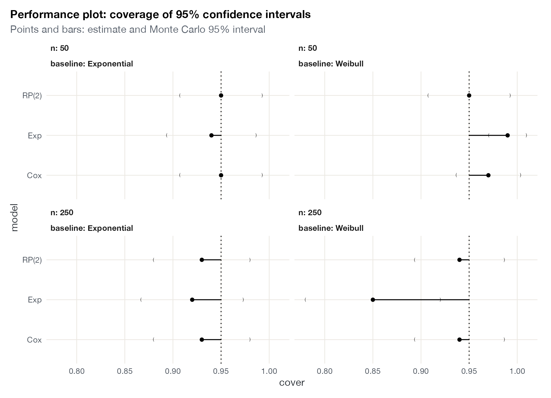
rsimsum::relhaz.
rsimsum::simsum() + autoplot() (shown); Stata simsum, siman
What it shows
Proof-of-concept papers for new synthesis methods, from MAIC and STC to NMI, ML-NMR, and ML-UMR, rest on simulation studies. Performance plots show a measure (bias, empirical standard error, coverage, mean squared error) for every method and scenario, together with its Monte Carlo standard error, so that readers can judge whether differences are real or simulation noise. The ML-UMR methods paper, for example, plots coverage with Monte Carlo error bars against a nominal 95% band.
How to read it
- Panels: scenarios (here sample size by baseline hazard).
- Rows: methods.
- Points and bars: estimated performance with Monte Carlo 95% intervals.
- Dotted line: the nominal value (95% coverage).
Interpretation
All three models achieve close to nominal coverage when the true baseline hazard is exponential. When it is Weibull and the sample size is 250, the misspecified exponential model’s coverage drops to 85% (Monte Carlo SE 3.6%), while the Cox and flexible parametric models stay near 94%. Misspecification shows up in coverage only once samples are large enough for bias to dominate the standard error.
Pitfalls
- Report the number of replications and Monte Carlo standard errors; with few replications apparent differences may be noise.
- Performance holds only for the simulated data-generating mechanisms.
- Coverage can be nominal for the wrong reason (for example, bias offset by overestimated standard errors); show bias and precision too.
Code
library(rsimsum)
library(ggplot2)
library(ggplot2)

# Simulation study of survival models (Cox, exponential, Weibull) across
# sample sizes and baseline hazards, shipped with rsimsum
data(relhaz)
s <- simsum(data = relhaz, estvarname = "theta", se = "se", true = -0.5,
            methodvar = "model", by = c("n", "baseline"))

# Coverage with Monte Carlo standard errors, by scenario and method
autoplot(summary(s), type = "lolly", stats = "cover") +
  ggplot2::labs(title = "Performance plot: coverage of 95% confidence intervals",
                subtitle = "Points and bars: estimate and Monte Carlo 95% interval")
References
- Morris TP, White IR, Crowther MJ. Using simulation studies to evaluate statistical methods. Stat Med. 2019;38:2074-2102. doi:10.1002/sim.8086
- Gasparini A. rsimsum: summarise results from Monte Carlo simulation studies. J Open Source Softw. 2018;3:739. doi:10.21105/joss.00739
- Chandler C, et al. Anchors away: navigating unanchored indirect comparisons with multilevel unanchored meta-regression. 2026. arXiv:2606.20341