Cumulative meta-analysis plot
Cumulative forest plot
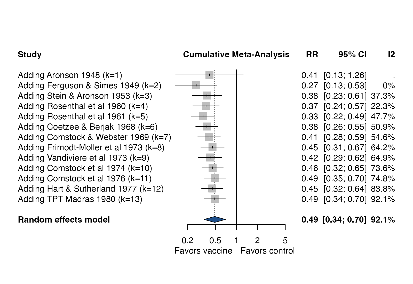
metadat::dat.bcg.
meta::metacum(), metafor::cumul(); Stata meta forestplot, cumulative()
What it shows
Each row of a cumulative forest plot is a complete meta-analysis of all studies up to and including that row. Ordered by publication year, it reconstructs the history of the evidence: when the pooled estimate stabilized, when it first became statistically significant, and whether later trials moved it. Ordered by precision or sample size, it becomes a check for small-study effects, since drift as smaller studies are added hints that they behave differently.
How to read it
- Rows: successive meta-analyses, labeled with the study just added and the running count \(k\).
- Squares and whiskers: the pooled estimate and 95% CI at that step (not the individual study result).
- Bottom diamond: the final pooled estimate, identical to the last row.
- Extra columns: running heterogeneity, such as \(I^2\).
Interpretation
The pooled risk ratio was already well below 1 after the first few trials of the 1940s and 1950s and has stayed there. What changed over time is heterogeneity: \(I^2\) climbed from 0% to 92% as trials from different latitudes were added. The history suggests the question shifted from “does BCG work” to “where does it work”.
Pitfalls
- Repeatedly testing a cumulative estimate inflates the type I error. A cumulative plot is descriptive; formal monitoring needs trial sequential analysis or a similar method.
- Choosing the ordering variable after looking at the data can tell a persuasive but post hoc story.
- Early rows rest on very few studies and random-effects estimates of \(\tau^2\) are unstable there.
Code
library(meta)

data(dat.bcg, package = "metadat")

m <- metabin(
  event.e = tpos, n.e = tpos + tneg,
  event.c = cpos, n.c = cpos + cneg,
  studlab = paste(author, year),
  data = dat.bcg, sm = "RR",
  common = FALSE, random = TRUE, method.tau = "REML"
)

# Add studies one at a time in order of publication year
cum <- metacum(m, sortvar = year)

forest(
  cum,
  label.left = "Favors vaccine", label.right = "Favors control",
  col.square = "#1d4e89", col.diamond = "#1d4e89",
  rightcols = c("effect", "ci", "I2"),
  rightlabs = c("RR", "95% CI", "I2")
)
meta esize tpos tneg cpos cneg, esize(lnrratio) random(reml)
meta forestplot, eform cumulative(year)References
- Lau J, Antman EM, Jimenez-Silva J, Kupelnick B, Mosteller F, Chalmers TC. Cumulative meta-analysis of therapeutic trials for myocardial infarction. N Engl J Med. 1992;327:248-254. doi:10.1056/NEJM199207233270406
- Clarke M, Brice A, Chalmers I. Accumulating research: a systematic account of how cumulative meta-analyses would have provided knowledge, improved health, reduced harm and saved resources. PLoS One. 2014;9:e102670. doi:10.1371/journal.pone.0102670