Trial sequential analysis plot
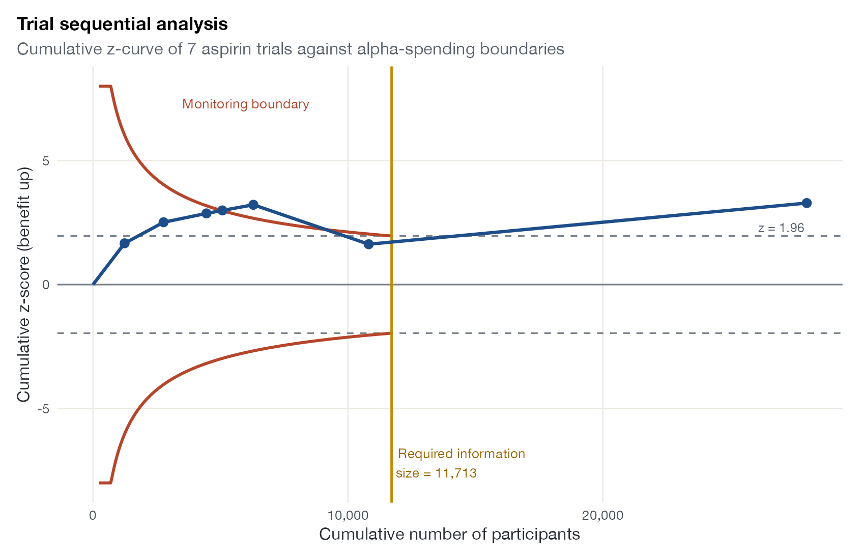
TSA plot, cumulative z-curve with monitoring boundaries
meta::Fleiss1993bin.
RTSA, custom ggplot2; Stata user-written tools
What it shows
Trial sequential analysis borrows group-sequential monitoring from single trials and applies it to a meta-analysis that is updated as trials appear. The cumulative z-curve is plotted against the number of participants (the information accrued). It is judged against monitoring boundaries that are strict early and relax toward the conventional 1.96 as the information approaches the required information size (RIS), the meta-analytic analogue of a trial’s sample size.
How to read it
- Horizontal axis: cumulative number of participants (or events, or statistical information).
- Vertical axis: cumulative z-score; here benefit is plotted upward.
- Blue curve: the z-statistic after each trial.
- Red curves: alpha-spending monitoring boundaries for benefit and harm.
- Dashed lines: the conventional \(z = \pm 1.96\) thresholds that ignore repeated testing.
- Vertical line: the required information size.
Interpretation
The z-curve crosses 1.96 after the second trial, when the monitoring boundary is still above 4, so that early signal is not conclusive. It reaches the boundary at the fourth trial (z = 2.99 against 2.98) and crosses it at the fifth, but the large AMIS trial then pulls it back to 1.63, below both thresholds. After ISIS-2 the information exceeds the required information size of about 11,700 participants and z = 3.29. Under these assumptions the evidence for benefit is firm, but it was not firm when the curve first crossed 1.96.
Pitfalls
- The RIS depends heavily on the anticipated effect, control risk, and heterogeneity adjustment. Report and justify them; choosing them after seeing the data defeats the purpose.
- The boundaries shown here use the simple O’Brien-Fleming approximation. Lan-DeMets spending functions and heterogeneity (diversity) adjustments give different boundaries.
- Trial sequential analysis is debated: meta-analyses are not planned experiments, and some methodologists argue for Bayesian or law-of-iterated-logarithm approaches instead.
- Crossing a boundary says nothing about bias or the certainty of the evidence.
Code
library(meta)
library(ggplot2)

# Aspirin after myocardial infarction: deaths in 7 trials (Fleiss 1993)
data(Fleiss1993bin)
d <- Fleiss1993bin[order(Fleiss1993bin$year), ]

# Cumulative common-effect (Mantel-Haenszel) z-statistics, benefit positive
cum <- metacum(metabin(d.asp, n.asp, d.plac, n.plac, studlab = study,
                       data = d, sm = "RR", common = TRUE, random = FALSE),
               pooled = "common")
k <- nrow(d)
z <- -cum$TE[1:k] / cum$seTE[1:k]
n <- cumsum(d$n.asp + d$n.plac)

# Required information size: control risk 10%, relative risk reduction 15%,
# two-sided alpha 5%, power 80%
pc <- 0.10; pe <- pc * 0.85; pbar <- (pc + pe) / 2
ris <- 4 * (qnorm(0.975) + qnorm(0.80))^2 * pbar * (1 - pbar) / (pc - pe)^2

# O'Brien-Fleming type monitoring boundary: z(t) = z_{alpha/2} / sqrt(t)
t <- seq(0.02, 1, length.out = 200)
bound <- data.frame(n = t * ris, z = pmin(qnorm(0.975) / sqrt(t), 8))

ggplot() +
  geom_hline(yintercept = c(-1.96, 1.96), linetype = "dashed", colour = "#7a828c") +
  geom_hline(yintercept = 0, colour = "#7a828c") +
  geom_line(data = bound, aes(n, z), colour = "#b5452b", linewidth = 1) +
  geom_line(data = bound, aes(n, -z), colour = "#b5452b", linewidth = 1) +
  geom_vline(xintercept = ris, colour = "#c28a00", linewidth = 0.8) +
  geom_line(data = data.frame(n = c(0, n), z = c(0, z)), aes(n, z),
            colour = "#1d4e89", linewidth = 1.1) +
  geom_point(data = data.frame(n, z), aes(n, z), colour = "#1d4e89", size = 2.6) +
  annotate("text", x = ris, y = -7.2, label = sprintf("Required information\nsize = %s", format(round(ris), big.mark = ",")),
           hjust = -0.05, size = 3.4, colour = "#9a6700") +
  annotate("text", x = 3500, y = 7.3, label = "Monitoring boundary", colour = "#b5452b", size = 3.4, hjust = 0) +
  annotate("text", x = 27000, y = 2.3, label = "z = 1.96", colour = "#5b636e", size = 3.2) +
  scale_x_continuous(labels = scales::comma) +
  coord_cartesian(ylim = c(-8, 8)) +
  labs(x = "Cumulative number of participants", y = "Cumulative z-score (benefit up)",
       title = "Trial sequential analysis",
       subtitle = "Cumulative z-curve of 7 aspirin trials against alpha-spending boundaries")
References
- Wetterslev J, Thorlund K, Brok J, Gluud C. Trial sequential analysis may establish when firm evidence is reached in cumulative meta-analysis. J Clin Epidemiol. 2008;61:64-75. doi:10.1016/j.jclinepi.2007.03.013
- Wetterslev J, Jakobsen JC, Gluud C. Trial Sequential Analysis in systematic reviews with meta-analysis. BMC Med Res Methodol. 2017;17:39. doi:10.1186/s12874-017-0315-7
- Lan KKG, DeMets DL. Discrete sequential boundaries for clinical trials. Biometrika. 1983;70:659-663. doi:10.1093/biomet/70.3.659