Residual versus fitted plot
Residual plot for meta-regression
metadat::dat.bcg.
metafor::rstandard(), fitted(); base R or ggplot2; Stata predict, residuals
What it shows
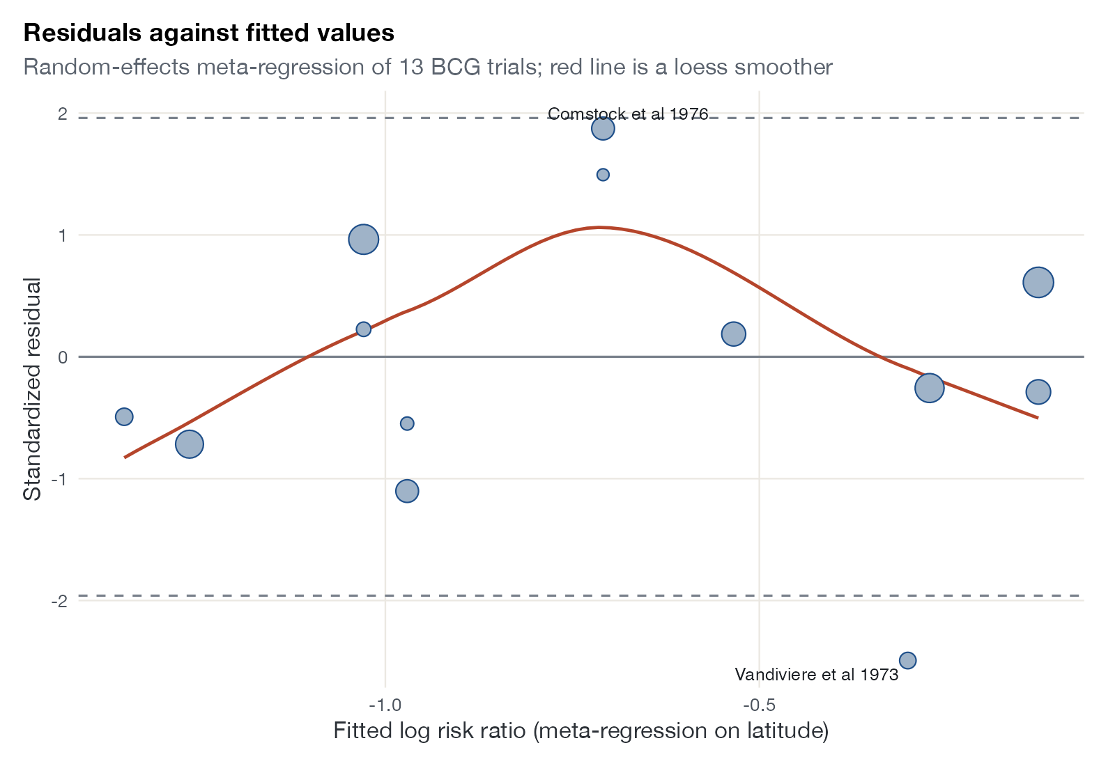
Any model that predicts study effects or patient outcomes from covariates, whether a meta-regression, an STC outcome model, a G-computation model, or the individual-level component of ML-NMR or ML-UMR, can be checked by plotting residuals against fitted values. If the model is adequate, residuals scatter randomly around zero with constant spread. Curvature suggests a missing nonlinear term; a funnel shape suggests the variance model is wrong; isolated large residuals are outliers.
How to read it
- Horizontal axis: fitted value from the model.
- Vertical axis: standardized (or deviance) residual.
- Reference lines: zero and ±1.96.
- Smoother: a loess curve that should be flat near zero.
- Point size: model weight.
Interpretation
Most residuals lie within ±1.96, but Vandiviere 1973 sits at −2.5 and Comstock 1976 near +1.9, and the smoother bends upward in the middle of the fitted range. With 13 studies, this is weak evidence of nonlinearity in latitude or of an unmodeled covariate, and a reason to look at those two trials.
Pitfalls
- With aggregate data, a clean residual plot cannot validate an individual-level functional form that the data cannot identify.
- With few studies, smoothers wiggle; do not over-read the curve.
- Residuals in random-effects models depend on how \(\tau^2\) is handled; state which residual is shown.
- In STC, residuals on the IPD used to fit the model say nothing about fit in the comparator population.
Code
library(metafor)
library(ggplot2)

data(dat.bcg, package = "metadat")
dat <- escalc(measure = "RR", ai = tpos, bi = tneg, ci = cpos, di = cneg,
              data = dat.bcg, slab = paste(author, year))

# Meta-regression on latitude, then standardized residuals against fitted values
fit <- rma(yi, vi, mods = ~ ablat, data = dat, method = "REML")
res <- data.frame(fitted = fitted(fit), resid = rstandard(fit)$z,
                  study = paste(dat$author, dat$year), w = weights(fit))

ggplot(res, aes(fitted, resid)) +
  geom_hline(yintercept = c(-1.96, 0, 1.96), linetype = c("dashed", "solid", "dashed"),
             colour = "#7a828c") +
  geom_smooth(method = "loess", formula = y ~ x, se = FALSE, span = 1,
              colour = "#b5452b", linewidth = 0.8) +
  geom_point(aes(size = w), shape = 21, fill = "#9fb3c8", colour = "#1d4e89") +
  ggrepel::geom_text_repel(data = subset(res, abs(resid) > 1.5), aes(label = study),
                           size = 3.2, colour = "#1b1f24") +
  scale_size_area(max_size = 7, guide = "none") +
  labs(x = "Fitted log risk ratio (meta-regression on latitude)",
       y = "Standardized residual",
       title = "Residuals against fitted values",
       subtitle = "Random-effects meta-regression of 13 BCG trials; red line is a loess smoother")
References
- Viechtbauer W, Cheung MWL. Outlier and influence diagnostics for meta-analysis. Res Synth Methods. 2010;1:112-125. doi:10.1002/jrsm.11
- Thompson SG, Higgins JPT. How should meta-regression analyses be undertaken and interpreted? Stat Med. 2002;21:1559-1573. doi:10.1002/sim.1187