Zip plot
Coverage zip plot of simulation confidence intervals
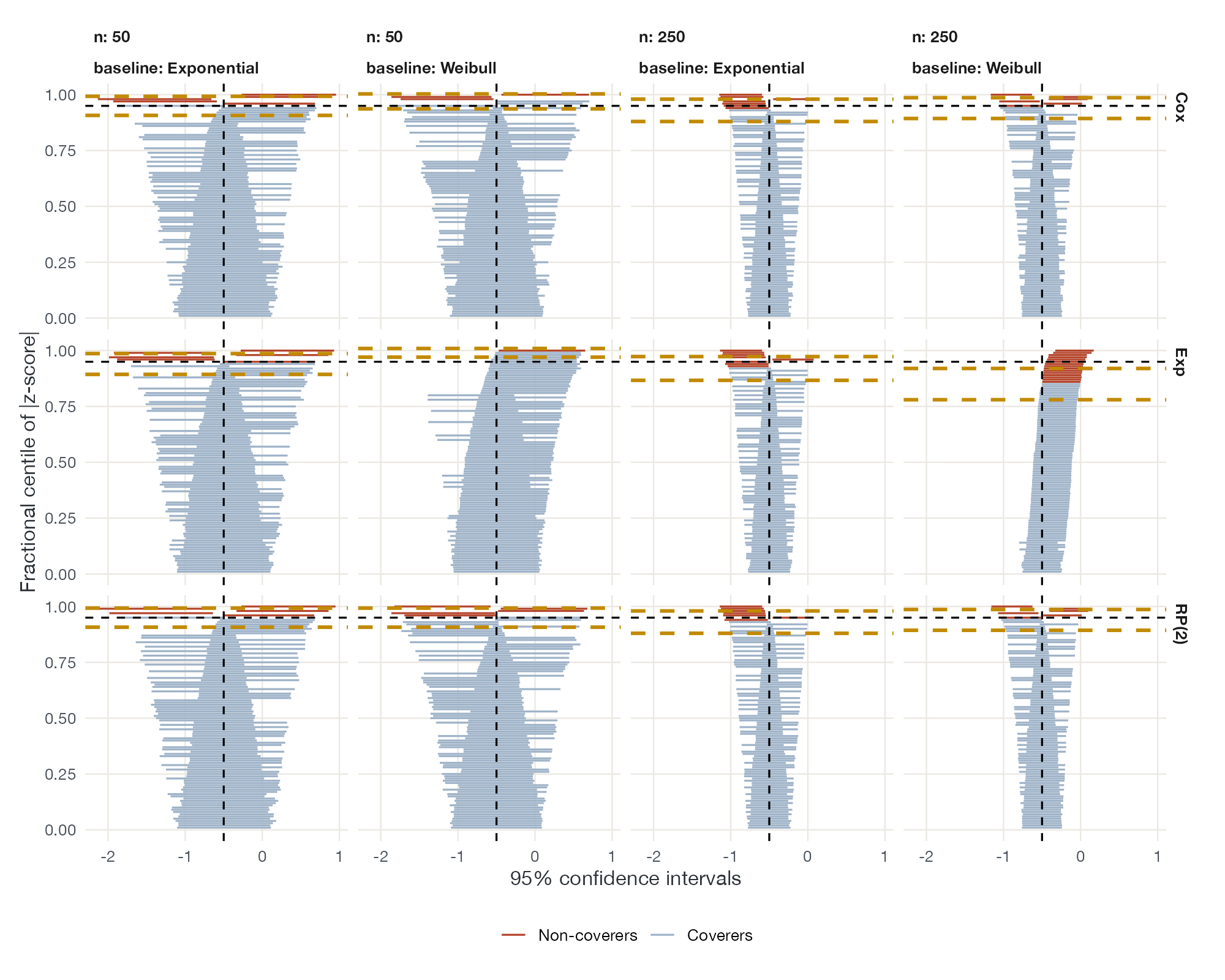
rsimsum::relhaz.
rsimsum::autoplot(type = "zip") (shown); Stata siman zipplot
What it shows
Morris, White, and Crowther proposed the zip plot to look inside a coverage estimate. Each replication’s confidence interval is drawn as a horizontal line, and the intervals are ranked by the centile of their \(|z|\) statistic for the true value. Intervals that miss the truth rise to the top. If the rank of the first noncovering interval sits at the nominal 95% line, coverage is right; the shape of the zipper also shows whether failures come from bias (intervals miss mostly on one side) or from standard errors that are too small.
How to read it
- Horizontal axis: estimate and confidence interval of each replication, with the true value marked.
- Vertical axis: fractional centile of \(|z|\) (rank).
- Colored band: noncovering intervals.
- Horizontal line near 95%: where noncoverage should begin if coverage were nominal.
Interpretation
For most scenarios the noncovering intervals start close to the 95% line and miss on both sides. For the exponential model with a Weibull baseline hazard and 250 patients, noncoverage begins well below 95% and the misses fall mostly on one side, so its undercoverage comes from bias rather than from underestimated standard errors.
Pitfalls
- Zip plots need the replication-level results, not only summaries.
- With few replications the display is coarse.
Code
library(rsimsum)
library(ggplot2)

data(relhaz)
s <- simsum(data = relhaz, estvarname = "theta", se = "se", true = -0.5,
            methodvar = "model", by = c("n", "baseline"), x = TRUE)

# Zip plot: every replication's confidence interval, ranked by how far it
# lies from the truth; noncovering intervals sit at the top
autoplot(s, type = "zip", zip_ci_colours = "#c28a00") +
  scale_colour_manual(values = c("Coverers" = "#9fb3c8", "Non-coverers" = "#b5452b"), name = NULL)
References
- Morris TP, White IR, Crowther MJ. Using simulation studies to evaluate statistical methods. Stat Med. 2019;38:2074-2102. doi:10.1002/sim.8086
- Gasparini A. rsimsum: summarise results from Monte Carlo simulation studies. J Open Source Softw. 2018;3:739. doi:10.21105/joss.00739