Posterior predictive distribution plot
Predictive density for a new study
MA
NMA
The posterior of the mean effect next to the posterior predictive distribution of the true effect in a new study.
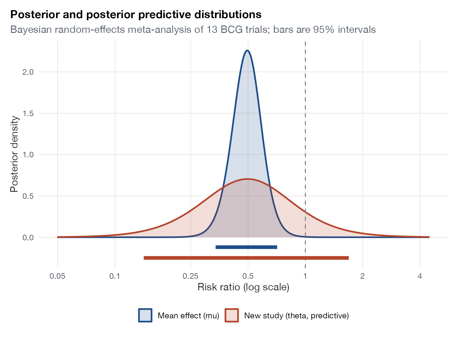
Bayesian random-effects meta-analysis of the 13 BCG trials (half-normal prior on tau with scale 0.5). Blue: posterior of the mean risk ratio. Red: posterior predictive distribution of the true risk ratio in a new trial. Bars are 95% intervals. Data:
metadat::dat.bcg.
Family
Model checking and Bayesian diagnostics
Purpose
Communicate the expected effect in a new setting, including between-study variation.
Inputs
Posterior of the mean effect and the heterogeneity parameter.
Software
R
bayesmeta ($dposterior(predict = TRUE)), brms, multinma::predict()
What it shows
The Bayesian analogue of the prediction interval plot. The posterior predictive distribution of \(\theta_{\text{new}}\) integrates over uncertainty in both the mean \(\mu\) and the heterogeneity \(\tau\), so it is wider and has heavier tails than a normal approximation using point estimates. For decisions about a specific setting, it is often the more relevant distribution.
How to read it
- Blue density and bar: posterior of the mean effect and its 95% credible interval.
- Red density and bar: predictive distribution of a new study’s true effect and its 95% interval.
- Dashed line: no effect.
- Area of the red curve right of the line: posterior predictive probability that a new setting sees no benefit.
Interpretation
The mean risk ratio is about 0.49 with a narrow posterior, but the predictive distribution spans roughly 0.14 to 1.7. A substantial share of its area lies above 1: in a new population, a lack of protection is entirely plausible even though the average benefit is certain.
Pitfalls
- The predictive distribution depends strongly on the prior for \(\tau\) when there are few studies.
- It describes study-level true effects, not individual patient outcomes.
- Exchangeability of the new setting with the observed studies is assumed, not tested.
Code
library(metafor)
library(bayesmeta)
library(ggplot2)

data(dat.bcg, package = "metadat")
dat <- escalc(measure = "RR", ai = tpos, bi = tneg, ci = cpos, di = cneg,
              data = dat.bcg)

bm <- bayesmeta(
  y = dat$yi, sigma = sqrt(dat$vi),
  labels = paste(dat$author, dat$year),
  mu.prior.mean = 0, mu.prior.sd = 4,
  tau.prior = function(t) dhalfnormal(t, scale = 0.5)
)

# Posterior of the mean effect mu versus the posterior predictive
# distribution of the true effect theta in a new study
x <- seq(-3, 1.5, length.out = 500)
d <- rbind(
  data.frame(x, density = bm$dposterior(mu = x), what = "Mean effect (mu)"),
  data.frame(x, density = bm$dposterior(theta = x, predict = TRUE),
             what = "New study (theta, predictive)")
)
ci <- bm$post.interval(mu.level = 0.95)
pi <- bm$post.interval(theta.level = 0.95, predict = TRUE)

ggplot(d, aes(x, density, colour = what, fill = what)) +
  geom_area(position = "identity", alpha = 0.18, linewidth = 0.9) +
  geom_vline(xintercept = 0, linetype = "dashed", colour = "#7a828c") +
  annotate("segment", x = ci[1], xend = ci[2], y = -0.12, yend = -0.12,
           colour = "#1d4e89", linewidth = 2) +
  annotate("segment", x = pi[1], xend = pi[2], y = -0.25, yend = -0.25,
           colour = "#b5452b", linewidth = 2) +
  scale_colour_manual(values = c("#1d4e89", "#b5452b"), name = NULL) +
  scale_fill_manual(values = c("#1d4e89", "#b5452b"), name = NULL) +
  scale_x_continuous(breaks = log(c(0.05, 0.1, 0.25, 0.5, 1, 2, 4)),
                     labels = c(0.05, 0.1, 0.25, 0.5, 1, 2, 4)) +
  labs(x = "Risk ratio (log scale)", y = "Posterior density",
       title = "Posterior and posterior predictive distributions",
       subtitle = "Bayesian random-effects meta-analysis of 13 BCG trials; bars are 95% intervals")
References
- Higgins JPT, Thompson SG, Spiegelhalter DJ. A re-evaluation of random-effects meta-analysis. J R Stat Soc Ser A. 2009;172:137-159. doi:10.1111/j.1467-985X.2008.00552.x
- Röver C. Bayesian random-effects meta-analysis using the bayesmeta R package. J Stat Softw. 2020;93(6):1-51. doi:10.18637/jss.v093.i06