Love plot
Standardized mean difference balance plot
maicplus::adsl_sat.
ggplot2 (shown); cobalt::love.plot() adaptations; maicplus::check_weights() for the numbers
What it shows
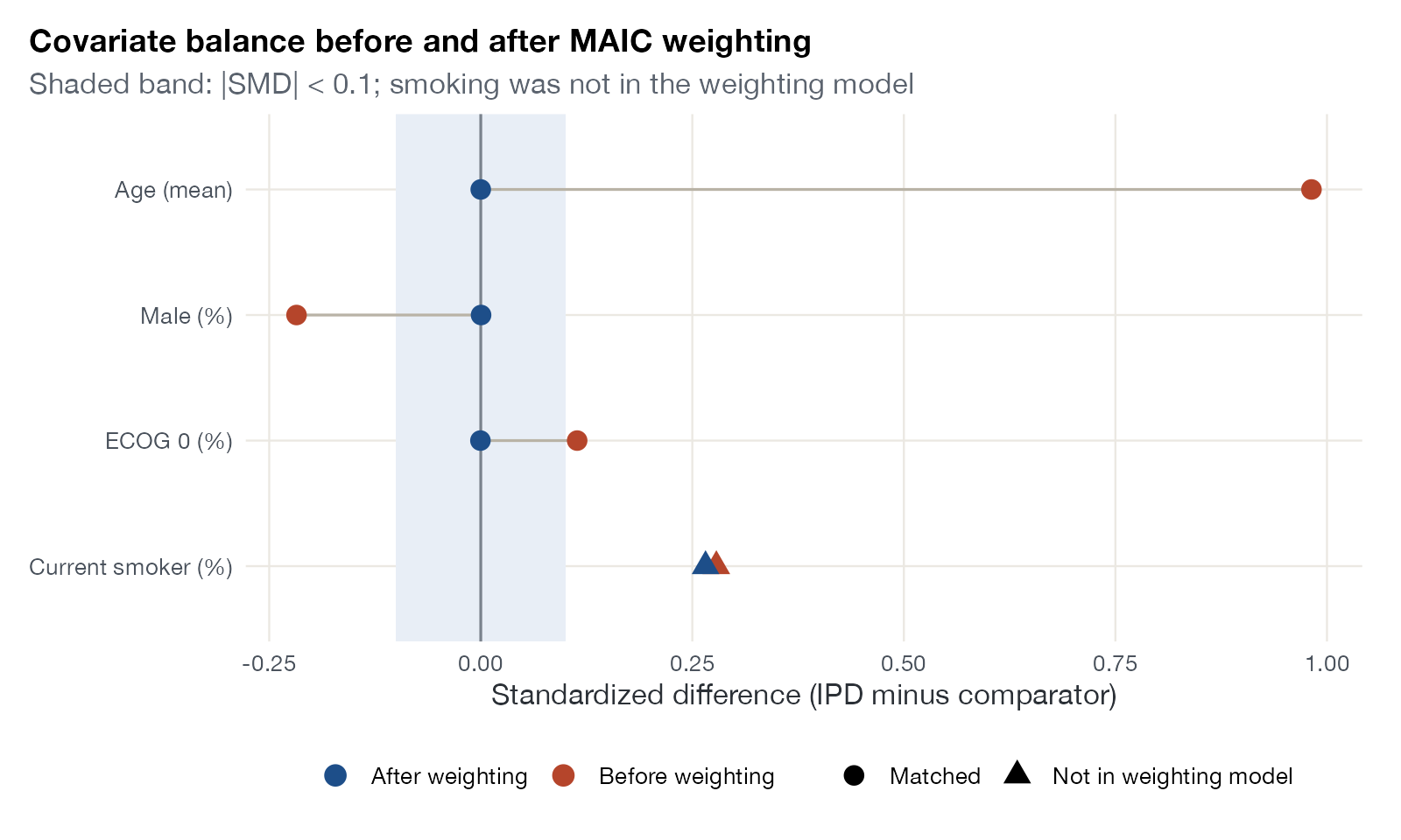
Borrowed from propensity score analysis, the Love plot shows, for each covariate, the standardized difference between the IPD and the target population before and after weighting. In MAIC it is the most common balance display. Its main value is less obvious than it seems: matched covariates are balanced exactly by construction, because the method of moments forces the weighted means to equal the targets.
How to read it
- Rows: covariates.
- Horizontal axis: standardized difference (IPD minus comparator, divided by the IPD standard deviation).
- Points: before (red) and after (blue) weighting; lines join them.
- Shape: whether the covariate was in the weighting model.
- Shaded band: a conventional ±0.1 region.
Interpretation
Before weighting, the IPD population is older by almost one standard deviation (age 59.8 against 51) and has fewer men. After weighting, age, sex, and ECOG differences are exactly zero, as they must be. Smoking, which was not matched, barely moves (0.28 before, 0.26 after): weighting on some covariates does not balance the others. If smoking modifies the treatment effect, this analysis is biased regardless of how good the matched rows look.
Pitfalls
- Zero differences for matched covariates verify the algorithm, not the validity of the comparison.
- Balance of means says nothing about balance of distributions; see the weighted covariate distribution plot.
- The plot cannot show balance on unreported or unmeasured effect modifiers, which is the central risk in population adjustment.
- The choice of standardizing SD (IPD, pooled, or comparator) changes the numbers; state it.
Code
library(maicplus)
library(ggplot2)

# Simulated single-arm IPD (N = 500) and published comparator means
data(adsl_sat)
target <- c(AGE = 51, SEX_MALE = 0.49, ECOG0 = 0.35, SMOKE = 0.19)

# Weight on age, sex, and ECOG only; smoking is deliberately left unmatched
ipd <- adsl_sat
ipd$AGE_CENTERED <- ipd$AGE - target[["AGE"]]
ipd$SEX_MALE_CENTERED <- ipd$SEX_MALE - target[["SEX_MALE"]]
ipd$ECOG0_CENTERED <- ipd$ECOG0 - target[["ECOG0"]]
w <- estimate_weights(ipd, centered_colnames = c("AGE_CENTERED", "SEX_MALE_CENTERED",
                                                 "ECOG0_CENTERED"))$data$weights

# Standardized differences (IPD minus target, scaled by the unweighted IPD SD)
smd <- function(x, t, wt) (weighted.mean(x, wt) - t) / sd(x)
bal <- do.call(rbind, lapply(names(target), function(v) data.frame(
  covariate = v,
  stage = c("Before weighting", "After weighting"),
  smd = c(smd(ipd[[v]], target[[v]], rep(1, nrow(ipd))), smd(ipd[[v]], target[[v]], w)),
  matched = ifelse(v == "SMOKE", "Not in weighting model", "Matched")
)))
bal$covariate <- factor(bal$covariate, levels = rev(names(target)),
                        labels = rev(c("Age (mean)", "Male (%)", "ECOG 0 (%)", "Current smoker (%)")))

ggplot(bal, aes(smd, covariate)) +
  annotate("rect", xmin = -0.1, xmax = 0.1, ymin = -Inf, ymax = Inf, fill = "#e8eef6") +
  geom_vline(xintercept = 0, colour = "#7a828c") +
  geom_line(aes(group = covariate), colour = "#b9b3a6") +
  geom_point(aes(colour = stage, shape = matched), size = 3.6) +
  scale_colour_manual(values = c("Before weighting" = "#b5452b", "After weighting" = "#1d4e89"),
                      name = NULL) +
  scale_shape_manual(values = c(Matched = 16, `Not in weighting model` = 17), name = NULL) +
  labs(x = "Standardized difference (IPD minus comparator)", y = NULL,
       title = "Covariate balance before and after MAIC weighting",
       subtitle = "Shaded band: |SMD| < 0.1; smoking was not in the weighting model") +
  guides(colour = guide_legend(order = 1), shape = guide_legend(order = 2))
References
- Signorovitch JE, Sikirica V, Erder MH, et al. Matching-adjusted indirect comparisons: a new tool for timely comparative effectiveness research. Value Health. 2012;15:940-947. doi:10.1016/j.jval.2012.05.004
- Phillippo DM, Ades AE, Dias S, Palmer S, Abrams KR, Welton NJ. NICE DSU Technical Support Document 18: Methods for population-adjusted indirect comparisons in submissions to NICE. 2016. sheffield.ac.uk/nice-dsu
- Austin PC, Stuart EA. Moving towards best practice when using inverse probability of treatment weighting (IPTW) using the propensity score to estimate causal treatment effects in observational studies. Stat Med. 2015;34:3661-3679. doi:10.1002/sim.6607