Posterior predictive check

PPC plot, replicated data check

NMA

ML-NMR

ML-UMR

Observed data against data replicated from the fitted Bayesian model, to check whether the model can reproduce what was seen.

MA NMA ML-NMR ML-UMREstablished

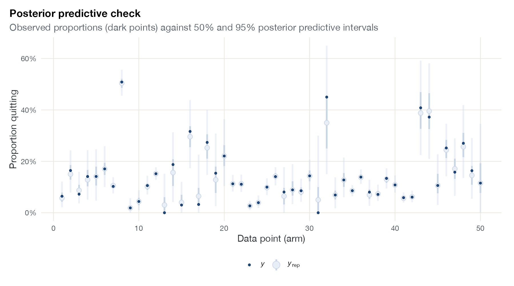
Posterior predictive check for a Bayesian random-effects NMA of smoking cessation: observed proportion quitting in each of 50 arms (dark points) against 50% and 95% intervals of 1,000 replicated datasets. Data: multinma::smoking.

Family

Model checking and Bayesian diagnostics

Purpose

Test whether the fitted model generates data that look like the observed data.

Inputs

Posterior draws of the fitted outcome for each data point.

Software

R bayesplot::ppc_intervals(), ppc_dens_overlay(); Python arviz.plot_ppc()

What it shows

A posterior predictive check simulates new data from the fitted model, once per posterior draw, and compares them with the observed data. If the model is adequate the observations look like typical replicates. Variants overlay densities of replicated and observed data, compare a test statistic across replicates, or, as here, place each observation within its predictive interval.

How to read it

Horizontal axis: data point (here each trial arm).
Vertical axis: outcome on its natural scale.
Light bars: 50% and 95% posterior predictive intervals.
Dark points: observed values.
Check: roughly 95% of points should fall inside the outer intervals, with no systematic pattern.

Interpretation

Nearly all observed quit proportions fall inside their 95% predictive intervals. The few near the edges are the zero-event arms already flagged by the residual deviance plot. The model reproduces the arm-level data well.

Pitfalls

A posterior predictive check uses the data twice (to fit and to check), so it is conservative; passing it is weak evidence.
It cannot test identifying assumptions that the data cannot inform, such as transitivity in NMA or no unmeasured effect modification in population adjustment.
Choose checks that target plausible failures (for example, extreme arms or heterogeneity), not only the mean.

Code

library(multinma)
library(bayesplot)

net <- set_agd_arm(smoking, study = studyn, trt = trtc, r = r, n = n,
                   trt_ref = "No intervention")

fit <- nma(net, trt_effects = "random",
           prior_intercept = normal(scale = 100),
           prior_trt = normal(scale = 100),
           prior_het = half_normal(scale = 5),
           seed = 2026)

# Replicate each arm's event count from the posterior predictive distribution
arms <- net$agd_arm
p <- sweep(as.matrix(fit, pars = "fitted_agd_arm"), 2, arms$.n, "/")
yrep <- t(apply(p[sample(nrow(p), 1000), ], 1, function(pr) rbinom(length(pr), arms$.n, pr)))

color_scheme_set(c("#e8eef6", "#c9d6e6", "#9fb3c8", "#5f82ab", "#1d4e89", "#12345c"))
ppc_intervals(y = arms$.r / arms$.n, yrep = sweep(yrep, 2, arms$.n, "/"),
              x = seq_along(arms$.r), prob = 0.5, prob_outer = 0.95) +
  ggplot2::scale_y_continuous(labels = scales::percent) +
  ggplot2::labs(x = "Data point (arm)", y = "Proportion quitting",
                title = "Posterior predictive check",
                subtitle = "Observed proportions (dark points) against 50% and 95% posterior predictive intervals")

import arviz as az

# idata: InferenceData with observed_data and posterior_predictive groups
az.plot_ppc(idata, kind="scatter", num_pp_samples=200)

References

Gelman A, Meng XL, Stern H. Posterior predictive assessment of model fitness via realized discrepancies. Stat Sin. 1996;6:733-807.
Gabry J, Simpson D, Vehtari A, Betancourt M, Gelman A. Visualization in Bayesian workflow. J R Stat Soc Ser A. 2019;182:389-402. doi:10.1111/rssa.12378
Röver C. Bayesian random-effects meta-analysis using the bayesmeta R package. J Stat Softw. 2020;93(6):1-51. doi:10.18637/jss.v093.i06