Effective sample size plot
ESS by weighting model or scenario
MAIC
Effective sample size after weighting, compared with the original sample size across weighting models or scenarios.
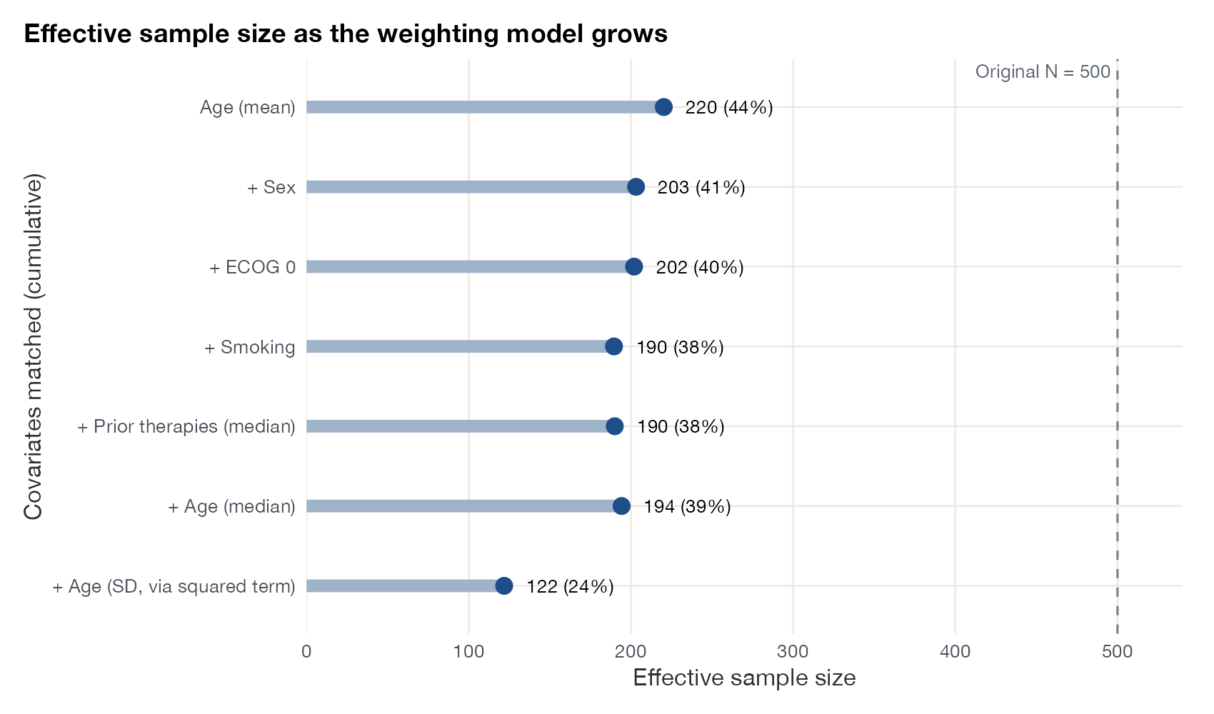
Effective sample size of simulated single-arm IPD (N = 500) as covariates are added to the MAIC weighting model one at a time. Data:
maicplus::centered_ipd_sat.
Family
Weighting, balance, and overlap
Purpose
Quantify the information lost to weighting and how it depends on the adjustment set.
Inputs
MAIC weights from one or more weighting models.
Software
Custom
ggplot2 (shown); maicplus::estimate_weights() reports the ESS
What it shows
The effective sample size of a weighted sample,
\[ \text{ESS} = \frac{(\sum_i w_i)^2}{\sum_i w_i^2}, \]
is the size of an unweighted sample that would give the same precision. Plotting it across weighting models, outcomes, or sensitivity scenarios shows how much information each adjustment costs and where the steep losses are.
How to read it
- Rows: weighting models, adding covariates cumulatively.
- Bar length: ESS, with the percentage of the original N.
- Dashed line: original sample size.
Interpretation
Matching mean age alone already reduces the ESS from 500 to 220, because the IPD are nine years older than the comparator population. Sex, ECOG, smoking, and prior therapies cost little more (ESS about 190). Matching the SD of age through a squared term drops the ESS to 122, a quarter of the original sample: the comparator’s age distribution is much narrower than the IPD’s.
Pitfalls
- There is no threshold at which an ESS becomes acceptable.
- The ESS depends on which covariates and moments are matched; a large ESS can come from leaving out an important effect modifier.
- Very small ESS makes robust sandwich variance estimates unreliable; prefer bootstrap intervals (see the bootstrap distribution plot).
Code
library(maicplus)
library(ggplot2)

data(centered_ipd_sat)

# Add covariates to the weighting model one at a time and record the ESS
steps <- list(
  "Age (mean)" = "AGE_CENTERED",
  "+ Sex" = "SEX_MALE_CENTERED",
  "+ ECOG 0" = "ECOG0_CENTERED",
  "+ Smoking" = "SMOKE_CENTERED",
  "+ Prior therapies (median)" = "N_PR_THER_MEDIAN_CENTERED",
  "+ Age (median)" = "AGE_MEDIAN_CENTERED",
  "+ Age (SD, via squared term)" = "AGE_SQUARED_CENTERED"
)
ess <- sapply(seq_along(steps), function(i) {
  estimate_weights(centered_ipd_sat, centered_colnames = unlist(steps[1:i]))$ess
})
d <- data.frame(model = factor(names(steps), levels = rev(names(steps))), ess = ess)

ggplot(d, aes(ess, model)) +
  geom_vline(xintercept = nrow(centered_ipd_sat), colour = "#7a828c", linetype = "dashed") +
  geom_segment(aes(x = 0, xend = ess, yend = model), colour = "#9fb3c8", linewidth = 3) +
  geom_point(size = 3.5, colour = "#1d4e89") +
  geom_text(aes(label = sprintf("%.0f (%.0f%%)", ess, 100 * ess / 500)), hjust = -0.25, size = 3.4) +
  annotate("text", x = 500, y = 7.45, label = "Original N = 500", hjust = 1.05, size = 3.3,
           colour = "#5b636e") +
  scale_x_continuous(limits = c(0, 540), expand = c(0, 0)) +
  labs(x = "Effective sample size", y = "Covariates matched (cumulative)",
       title = "Effective sample size as the weighting model grows")
References
- Phillippo DM, Ades AE, Dias S, Palmer S, Abrams KR, Welton NJ. NICE DSU Technical Support Document 18: Methods for population-adjusted indirect comparisons in submissions to NICE. 2016. sheffield.ac.uk/nice-dsu
- Remiro-Azócar A, Heath A, Baio G. Methods for population adjustment with limited access to individual patient data: a review and simulation study. Res Synth Methods. 2021;12:750-775. doi:10.1002/jrsm.1511