Joint posterior plot of effect and heterogeneity
Bivariate posterior of mu and tau
metadat::dat.bcg.
bayesmeta::plot(which = 2)
What it shows
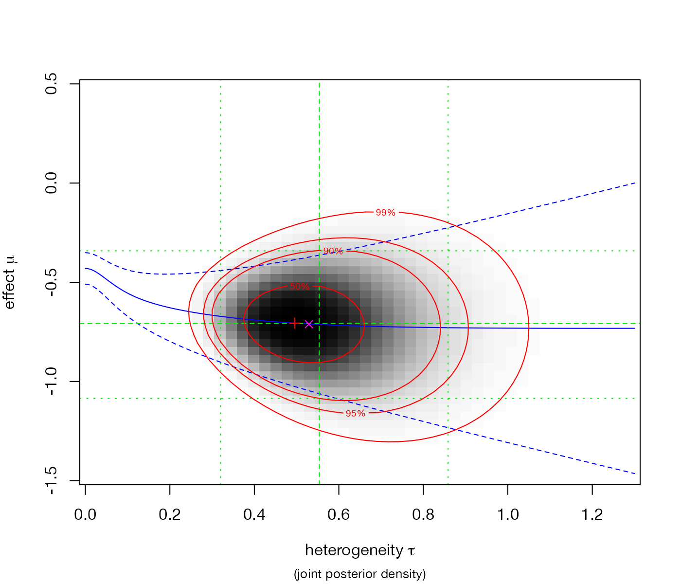
In the normal-normal hierarchical model the two key parameters are correlated in an informative way: the mean \(\mu\) and its uncertainty depend on how large the heterogeneity \(\tau\) is. The joint posterior plot shows the two-dimensional density with credible regions, together with the conditional mean of \(\mu\) at each value of \(\tau\) and its interval. It explains why random-effects results can be sensitive to how \(\tau\) is estimated.
How to read it
- Horizontal axis: heterogeneity SD \(\tau\).
- Vertical axis: mean effect \(\mu\).
- Gray shading: joint posterior density.
- Red contours: 90%, 95%, and 99% credible regions.
- Blue lines: conditional posterior mean of \(\mu\) given \(\tau\), with 95% interval.
- Green lines: marginal posterior medians and 95% intervals.
Interpretation
The posterior mass lies between \(\tau \approx 0.3\) and 0.9, well away from zero, so heterogeneity is certain. The conditional mean of \(\mu\) is nearly flat across that range, but its interval fans out as \(\tau\) grows. The point estimate is robust to the heterogeneity estimate; its uncertainty is not.
Pitfalls
- The shape depends on the priors, particularly for \(\tau\) when there are few studies.
- This display is specific to two-parameter models; with covariates or networks, look at pairwise plots of key parameters instead.
Code
library(metafor)
library(bayesmeta)

data(dat.bcg, package = "metadat")
dat <- escalc(measure = "RR", ai = tpos, bi = tneg, ci = cpos, di = cneg,
              data = dat.bcg)

bm <- bayesmeta(
  y = dat$yi, sigma = sqrt(dat$vi),
  labels = paste(dat$author, dat$year),
  mu.prior.mean = 0, mu.prior.sd = 4,
  tau.prior = function(t) dhalfnormal(t, scale = 0.5)
)

# Joint posterior density of (mu, tau): contours of 90%, 95%, 99% credible
# regions, with the conditional mean of mu given tau
plot(bm, which = 2, main = "", taulim = c(0, 1.3), mulim = c(-1.5, 0.5))
References
- Röver C. Bayesian random-effects meta-analysis using the bayesmeta R package. J Stat Softw. 2020;93(6):1-51. doi:10.18637/jss.v093.i06
- Friede T, Röver C, Wandel S, Neuenschwander B. Meta-analysis of few small studies in orphan diseases. Res Synth Methods. 2017;8:79-91. doi:10.1002/jrsm.1217