Multidimensional scaling ranking plot
MDS rank plot
netmeta::Linde2015.
mdsrank; R cmdscale() with ggplot2 (shown)
What it shows
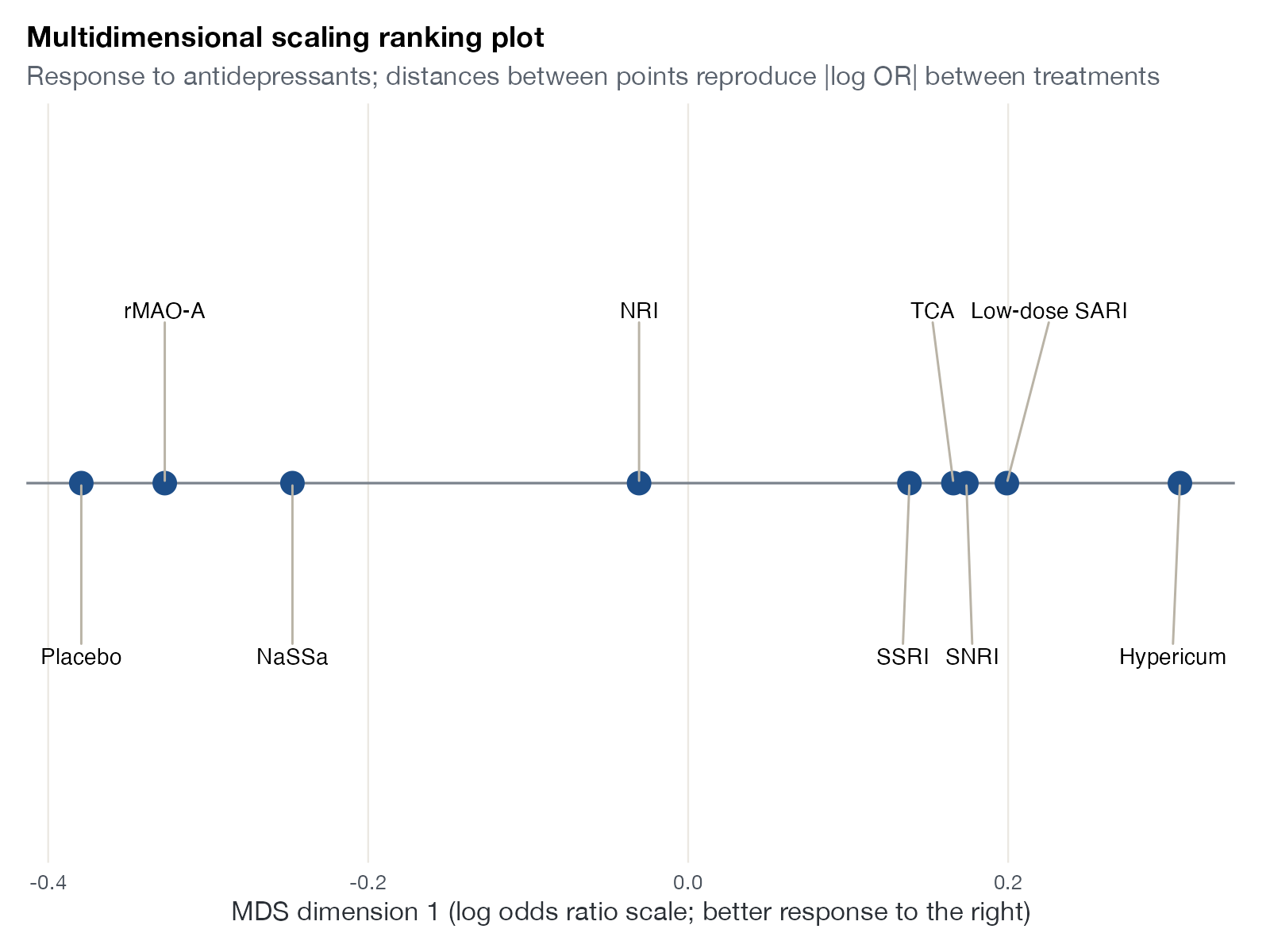
Chung and Lumley suggested multidimensional scaling for exploring network meta-analysis data. Stata’s mdsrank applies it to the matrix of pairwise relative effects and plots treatments on the resulting dimension. Unlike a ranking, the positions keep the distances: treatments that are close on the axis have similar effects. Under a consistency model the pairwise effects are exactly one-dimensional, so a single axis reproduces them; with inconsistent evidence (for example, direct estimates only) more dimensions appear.
How to read it
- Horizontal axis: the first MDS dimension, on the scale of the effect measure.
- Points: treatments; distances approximate absolute pairwise effects.
- Direction: oriented here so that better response lies to the right.
Interpretation
Hypericum sits furthest right. Low-dose SARI, TCA, SNRI, and SSRI form a tight cluster, so their ranking among themselves has little practical meaning. NaSSa, rMAO-A, and placebo sit apart at the left, with NRI in between.
Pitfalls
- MDS reproduces point estimates only; uncertainty is not shown.
- The sign and origin of the axis are arbitrary.
- Additional dimensions, if any, are hard to interpret clinically.
Code
library(netmeta)

# Antidepressants in primary care (Linde et al. 2015): arm-level binary outcomes
data(Linde2015)
d <- Linde2015
nma_for <- function(v, small) {
  p <- pairwise(treat = list(d$treatment1, d$treatment2, d$treatment3),
                event = list(d[[paste0(v, 1)]], d[[paste0(v, 2)]], d[[paste0(v, 3)]]),
                n = list(d$n1, d$n2, d$n3), studlab = d$id, sm = "OR", allstudies = TRUE)
  netmeta(p, common = FALSE, reference.group = "Placebo", small.values = small)
}
library(ggplot2)

resp <- nma_for("resp", small = "undesirable")

# Classical multidimensional scaling of the matrix of absolute pairwise
# log odds ratios. Under a consistency model the distances are exactly
# one-dimensional, so the first dimension orders the treatments
dist <- abs(resp$TE.random)
mds <- cmdscale(dist, k = 1)
pts <- data.frame(treatment = rownames(mds), dim1 = mds[, 1])
# Orient the dimension so that better treatments lie to the right
if (cor(pts$dim1, resp$TE.random[pts$treatment, "Placebo"]) < 0) pts$dim1 <- -pts$dim1
pts$side <- ifelse(rank(pts$dim1) %% 2 == 0, 1, -1)

ggplot(pts, aes(dim1, 0)) +
  geom_hline(yintercept = 0, colour = "#7a828c") +
  geom_point(size = 4.5, colour = "#1d4e89") +
  ggrepel::geom_text_repel(aes(label = treatment), nudge_y = 0.25 * pts$side,
                           direction = "x", size = 3.6, segment.colour = "#b9b3a6") +
  scale_y_continuous(limits = c(-0.5, 0.5), breaks = NULL) +
  labs(x = "MDS dimension 1 (log odds ratio scale; better response to the right)", y = NULL,
       title = "Multidimensional scaling ranking plot",
       subtitle = "Response to antidepressants; distances between points reproduce |log OR| between treatments") +
  theme(panel.grid.major.y = element_blank())
network meta consistency
mdsrank, best(max) labels(...)References
- Chung H, Lumley T. Graphical exploration of network meta-analysis data: the use of multidimensional scaling. Clin Trials. 2008;5:301-307. doi:10.1177/1740774508093614
- Chaimani A, Higgins JPT, Mavridis D, Spyridonos P, Salanti G. Graphical tools for network meta-analysis in STATA. PLoS One. 2013;8:e76654. doi:10.1371/journal.pone.0076654