Subgroup data availability matrix

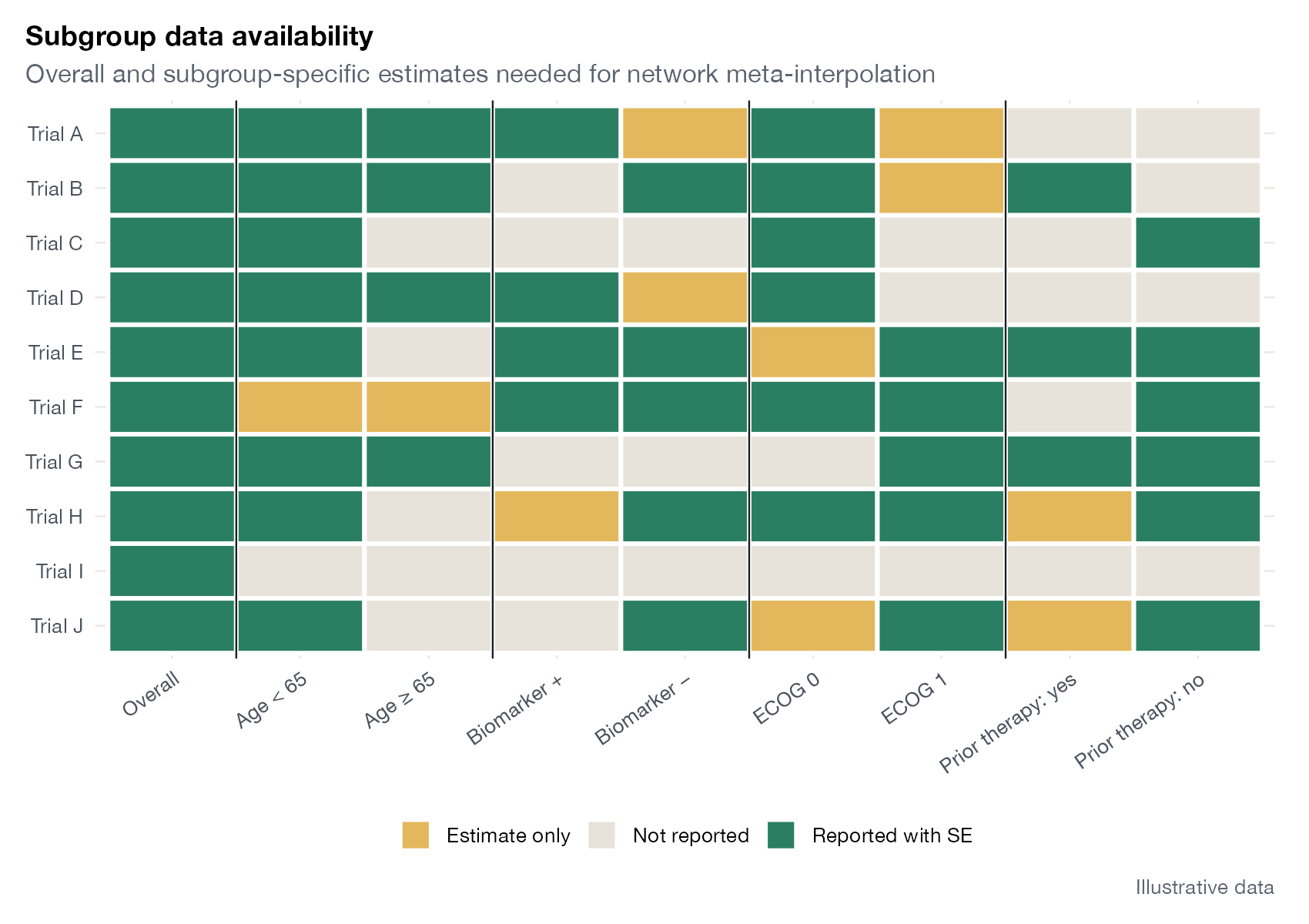
Subgroup reporting heat map

A trial-by-subgroup grid showing which overall and subgroup-specific estimates are reported, and whether they come with standard errors.

NMIML-NMRProposed

Availability of overall and subgroup-specific estimates for four candidate effect modifiers across ten trials. Green: estimate with standard error; amber: estimate only; gray: not reported. Illustrative data.

Family

Network meta-interpolation

Purpose

Check whether the subgroup evidence needed for NMI (or other adjustments) exists before analysis.

Inputs

Extraction records of reported overall and subgroup results.

Software

Custom ggplot2 (shown)

What it shows

NMI depends directly on subgroup results. A study-by-subgroup matrix, colored by what each trial reports, shows before any analysis whether the evidence can support the method and which effect modifiers can realistically be adjusted for. It also exposes selective subgroup reporting, which can itself bias an analysis that relies on reported subgroups.

How to read it

• Rows: trials.
• Columns: the overall estimate and the levels of each candidate effect modifier.
• Colors: reported with standard error, estimate only, or not reported.

Interpretation

Every trial reports an overall effect, but subgroup reporting is patchy. Age is the most complete modifier, yet only four trials report both age subgroups with standard errors; for the biomarker, ECOG status, and prior therapy only two trials do, and Trial I reports no subgroups at all. Any NMI here would have to drop trials or impute missing subgroup results, and the analysis should say which.

Pitfalls

• A subgroup that is “reported” may still use different cutpoints across trials.
• Missingness may be informative: trials often report subgroups that look interesting.
• The matrix documents availability, not quality or credibility of the subgroup analyses.

Code

R

library(ggplot2)

# Which trials report overall and subgroup results for each candidate effect
# modifier? Illustrative data for a 10-trial network.
set.seed(8)
trials <- paste("Trial", LETTERS[1:10])
items <- c("Overall", "Age < 65", "Age ≥ 65", "Biomarker +", "Biomarker −",
           "ECOG 0", "ECOG 1", "Prior therapy: yes", "Prior therapy: no")
status <- matrix(sample(c("Reported with SE", "Estimate only", "Not reported"),
                        length(trials) * length(items), replace = TRUE,
                        prob = c(0.6, 0.15, 0.25)), nrow = length(trials))
status[, 1] <- "Reported with SE"
status[c(3, 7), 4:5] <- "Not reported"
status[9, 2:9] <- "Not reported"
d <- data.frame(trial = rep(trials, length(items)), item = rep(items, each = length(trials)),
                status = as.vector(status))
d$item <- factor(d$item, levels = items)
d$trial <- factor(d$trial, levels = rev(trials))

ggplot(d, aes(item, trial, fill = status)) +
  geom_tile(colour = "white", linewidth = 1) +
  geom_vline(xintercept = c(1.5, 3.5, 5.5, 7.5), colour = "#1b1f24", linewidth = 0.4) +
  scale_fill_manual(values = c("Reported with SE" = "#2a7f62", "Estimate only" = "#e3b85c",
                               "Not reported" = "#e7e3db"), name = NULL) +
  labs(x = NULL, y = NULL, title = "Subgroup data availability",
       subtitle = "Overall and subgroup-specific estimates needed for network meta-interpolation",
       caption = "Illustrative data") +
  theme(axis.text.x = element_text(angle = 35, hjust = 1), panel.grid = element_blank())

References

• Harari O, Soltanifar M, Cappelleri JC, et al. Network meta-interpolation: effect modification adjustment in network meta-analysis using subgroup analyses. Res Synth Methods. 2023;14:211-233. doi:10.1002/jrsm.1608