Rankogram
Rank probability plot
NMA
ML-NMR
For each treatment, the probability of occupying each rank from best to worst.
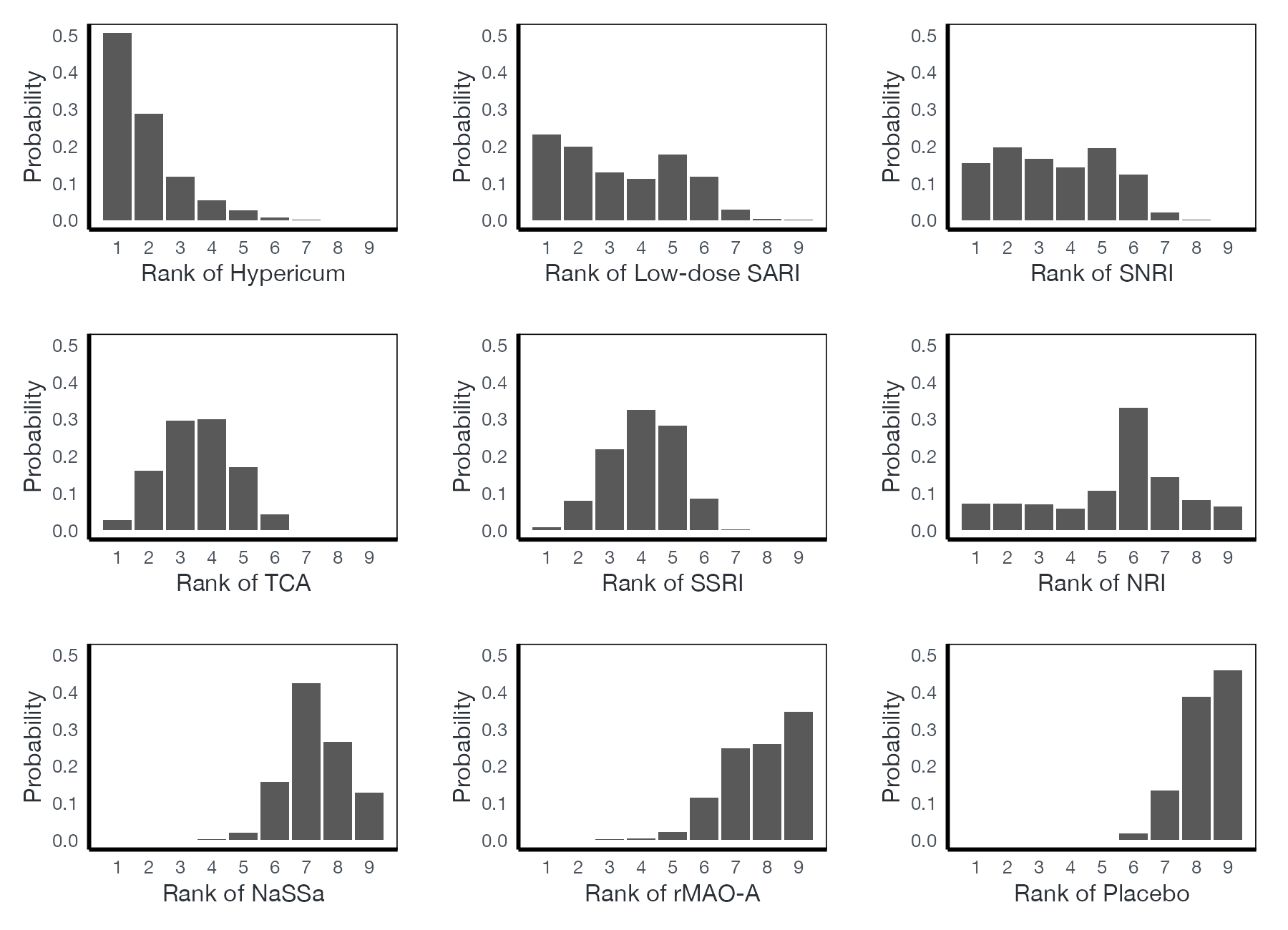
Rankograms for response in the antidepressant network (nine treatments, random effects), from 5,000 resamples of the network estimates. Data:
netmeta::Linde2015.
Family
Treatment ranking
Purpose
Show the full uncertainty in treatment rankings.
Inputs
Rank probabilities from Bayesian posterior draws or frequentist resampling.
Software
R
netmeta::rankogram(), multinma::posterior_rank_probs(), gemtc; Stata sucra
What it shows
A ranking summary such as SUCRA reduces a whole distribution to one number. The rankogram shows the distribution itself: for every treatment, the probability that it is the best, second best, and so on. Broad or multimodal rank distributions reveal ranking uncertainty that a single score hides.
How to read it
- One panel (or line) per treatment.
- Horizontal axis: rank, from 1 (best) to the number of treatments.
- Vertical axis: probability of that rank.
- Shape: a single tall bar means the rank is certain; a flat profile means it is not.
Interpretation
Hypericum has about a 50% chance of being the best treatment for response, but also a meaningful chance of ranks 2 to 4. Low-dose SARI and SNRI spread their probability over ranks 1 to 6. Placebo, rMAO-A, and NaSSa concentrate on the bottom ranks. The data separate the bottom of the ranking much more clearly than the top.
Pitfalls
- Rank probabilities say nothing about the size of the differences; two treatments can swap ranks with a clinically trivial difference.
- The probability of being best favors treatments with imprecise estimates, which have more mass in the tails.
- Ranks are relative to the treatments in the network; adding or removing a treatment changes them.
- Always report relative effects alongside rankings.
Code
library(netmeta)

# Antidepressants in primary care (Linde et al. 2015): arm-level binary outcomes
data(Linde2015)
d <- Linde2015
nma_for <- function(v, small) {
  p <- pairwise(treat = list(d$treatment1, d$treatment2, d$treatment3),
                event = list(d[[paste0(v, 1)]], d[[paste0(v, 2)]], d[[paste0(v, 3)]]),
                n = list(d$n1, d$n2, d$n3), studlab = d$id, sm = "OR", allstudies = TRUE)
  netmeta(p, common = FALSE, reference.group = "Placebo", small.values = small)
}

resp <- nma_for("resp", small = "undesirable")

# Probability of each rank for each treatment (resampling from the NMA)
rk <- rankogram(resp, nsim = 5000)
plot(rk)
network meta consistency
network rank max, all zero reps(5000) gen(prob)
sucra prob*, rankogram lab(...)References
- Salanti G, Ades AE, Ioannidis JPA. Graphical methods and numerical summaries for presenting results from multiple-treatment meta-analysis: an overview and tutorial. J Clin Epidemiol. 2011;64:163-171. doi:10.1016/j.jclinepi.2010.03.016
- Mbuagbaw L, Rochwerg B, Jaeschke R, et al. Approaches to interpreting and choosing the best treatments in network meta-analyses. Syst Rev. 2017;6:79. doi:10.1186/s13643-017-0473-z
- Linde K, Kriston L, Rücker G, et al. Efficacy and acceptability of pharmacological treatments for depressive disorders in primary care: systematic review and network meta-analysis. Ann Fam Med. 2015;13:69-79. doi:10.1370/afm.1687