Fitting, priors, and diagnostics

library(mlumr)
library(ggplot2)
options(mc.cores = parallel::detectCores())

This vignette covers the mechanics of fitting an ML-UMR model with mlumr(): sampler control, backends, priors, inspecting a fit, and MCMC diagnostics. It is family-agnostic, we illustrate with the real plaque-psoriasis binary example from vignette("binary-outcomes"), but the workflow is identical for continuous, count, and survival outcomes. For which method to report, see vignette("choosing-a-method").

mlumr() fits two model variants by Stan: model = "spfa" (shared prognostic-factor coefficients) and model = "relaxed" (treatment-specific coefficients, allowing effect modification). The default backend is rstan; cmdstanr is an optional alternative. The sampler messages, timings and Engine: line shown throughout this vignette were produced with cmdstanr, which vignettes/precompile.R selects, so running the same code with the defaults prints rstan’s equivalents instead.

A model to work with

We reuse the plaque-psoriasis binary example, a compact ML-UMR fit that the rest of this vignette inspects, tunes, and diagnoses (the data preparation is covered in vignette("binary-outcomes")).

Hypothetical single-arm trials. UNCOVER-2 and FIXTURE are randomized trials. Dropping their common reference arms (placebo and etanercept) turns them into hypothetical single-arm trials and leaves fully disconnected evidence; we do this only to illustrate ML-UMR. In practice, randomized trials should never be analyzed this way: ML-NMR (for example with multinma) or another appropriate method should be used for them. ML-UMR should only be used for fully unanchored, single-arm comparisons.

data("psoriasis_ipd")   # bundled with mlumr (from multinma, GPL-3)
data("psoriasis_agd")

covs <- c("age", "bsa", "weight")
ipd <- psoriasis_ipd
ipd$bsa <- ipd$bsa / 100          # body-surface area: % -> proportion
ipd <- ipd[ipd$study == "UNCOVER-2" & ipd$treatment == "IXE_Q4W", ]
ipd <- ipd[stats::complete.cases(ipd[, c("pasi75", covs)]), ]

agd <- psoriasis_agd
agd$bsa_mean <- agd$bsa_mean / 100; agd$bsa_sd <- agd$bsa_sd / 100
agd <- agd[agd$study == "FIXTURE" & agd$treatment == "SEC_300", ]

dat <- combine_data(
  set_ipd(ipd, treatment = "treatment", outcome = "pasi75", covariates = covs),
  set_agd(agd, treatment = "treatment", outcome_n = "pasi75_n", outcome_r = "pasi75_r",
          cov_means = c("age_mean", "bsa_mean", "weight_mean"),
          cov_sds   = c("age_sd", "bsa_sd", "weight_sd"),
          cov_types = c("continuous", "continuous", "continuous")))
dat <- add_integration(dat, n_int = 64,
  age    = distr(qgamma,     mean = age_mean,    sd = age_sd),
  bsa    = distr(qlogitnorm, mean = bsa_mean,    sd = bsa_sd),
  weight = distr(qgamma,     mean = weight_mean, sd = weight_sd))

fit <- mlumr(dat, model = "spfa",
             prior_beta = prior_normal(0, 2.5, autoscale = TRUE),
             chains = 4, iter = 2000, warmup = 1000, seed = 2026, refresh = 0)
#> Running MCMC with 4 parallel chains...
#> 
#> Chain 2 finished in 1.3 seconds.
#> Chain 3 finished in 1.3 seconds.
#> Chain 4 finished in 1.2 seconds.
#> Chain 1 finished in 1.4 seconds.
#> 
#> All 4 chains finished successfully.
#> Mean chain execution time: 1.3 seconds.
#> Total execution time: 1.6 seconds.

Controlling the sampler

All sampler controls are arguments to mlumr(). For a production analysis use more chains and iterations than the short settings above:

fit <- mlumr(
  dat, model = "spfa",
  chains = 4,            # number of MCMC chains
  iter = 4000,           # total iterations per chain
  warmup = 2000,         # warmup iterations
  seed = 2026,           # reproducibility
  adapt_delta = 0.99,    # raise toward 1 to remove divergences
  max_treedepth = 15,    # raise if treedepth is saturated
  refresh = 500          # progress printing (0 = silent)
)

Backend selection

rstan (default) uses the model compiled into the installed package. cmdstanr is an optional backend, selected per fit or globally with mlumr_engine("cmdstanr"):

fit_cmd <- mlumr(dat, model = "spfa", engine = "cmdstanr", seed = 2026, refresh = 0)

cmdstanr is often faster once compiled, especially with parallel chains and long runs. Posterior estimates agree up to Monte Carlo error.

Priors

The defaults, prior_normal(0, 10) for intercepts and prior_normal(0, 2.5) for regression coefficients, are generic starting values rather than calibrated choices for every family and outcome scale. Autoscaling divides a coefficient prior’s location and scale by each covariate’s SD so its intended contribution is preserved when predictors use different units. For family = "normal" the intercepts, the identity-link coefficients and the residual SD are in the outcome’s own units, so there the defaults and autoscaled scales are also multiplied by the IPD outcome SD (see vignette("continuous-outcomes")). Inspect the priors actually passed to Stan, including autoscaled scales, with prior_summary():

prior_summary(fit)
#> Priors for ML-UMR Fit
#> =====================
#> 
#> Intercepts (mu_index, mu_comparator):
#>   normal(0, 10)
#>   (package default, mlumr 0.1.0.9000)
#> 
#> Regression coefficients (beta):
#>   Family: normal
#>  coefficient mean  scale autoscaled   sd_x
#>          age    0  0.196       TRUE 12.784
#>          bsa    0 14.055       TRUE  0.178
#>       weight    0  0.120       TRUE 20.794
#>   (scale = user_scale / sd_x for autoscaled rows)

Overlaying the prior on the posterior shows how much the data have updated each parameter, the intercepts move sharply away from their \mathrm{N}(0,10) prior:

plot_prior_posterior(fit, pars = c("mu_index", "mu_comparator"))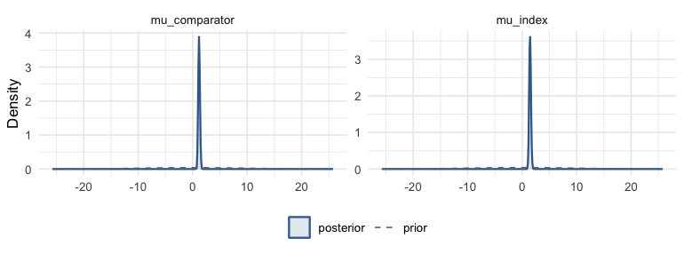

plot of chunk prior-post

Inspecting a fit

print() gives a one-line description of the model; summary() tabulates the posterior for every parameter (point estimate, credible interval, and the per-parameter convergence diagnostics):

print(fit)
#> ML-UMR Fit
#> ==========
#> 
#> Model: SPFA (Shared Prognostic Factors) 
#> Family: Binary 
#> Link: logit 
#> Engine: cmdstanr 
#> Treatments:
#>   Index (IPD): IXE_Q4W 
#>   Comparator (AgD): SEC_300 
#> 
#> Data:
#>   IPD: n = 345 observations
#>   AgD: 1 rows
#>   Covariates: 3 
#>   Integration points: 64 
#> 
#> Sampling:
#>   Chains: 4 
#>   Iterations: 2000 (warmup: 1000 )
#> 
#> Key Parameters:
#>        variable       mean         sd        2.5%     97.5%      Rhat
#>        mu_index 1.44618427 0.15636550  1.15196094 1.7651909 0.9995392
#>   mu_comparator 1.17260184 0.15224510  0.88731421 1.4799876 1.0000963
#>       lor_index 0.25377673 0.20530813 -0.15266887 0.6555978 1.0012879
#>  lor_comparator 0.25466793 0.20617373 -0.15273282 0.6587242 1.0013579
#>        rd_index 0.04763409 0.03873935 -0.02809253 0.1234016 1.0017769
#>   rd_comparator 0.04156580 0.03362521 -0.02554187 0.1053535 1.0015519
#> 
#> Use summary() for full results
summary(fit)
#> ML-UMR Model Summary
#> ====================
#> 
#> Model: SPFA 
#> Family: Binary 
#> Link: logit 
#> Engine: cmdstanr 
#> Treatments: IXE_Q4W (IPD) vs SEC_300 (AgD)
#> 
#> MCMC Diagnostics:
#>   Divergent transitions: 0 
#>   Max treedepth hits: 0 
#>   Max Rhat: 1.004 
#>   Min ESS: 1890 
#> 
#> Intercepts (logit scale):
#>       variable     mean        sd      2.5%    97.5%      Rhat
#>       mu_index 1.446184 0.1563655 1.1519609 1.765191 0.9995392
#>  mu_comparator 1.172602 0.1522451 0.8873142 1.479988 1.0000963
#> 
#> Regression Coefficients:
#>      variable        mean          sd        2.5%        97.5%      Rhat
#>     beta[age] -0.04072437 0.010852931 -0.06213992 -0.020515311 1.0013211
#>     beta[bsa]  0.09474860 0.738994077 -1.31835682  1.580247738 1.0015116
#>  beta[weight] -0.01462932 0.006335175 -0.02729679 -0.002487916 0.9998753
#> 
#> Marginal Treatment Effects:
#>   Log Odds Ratios:
#>        variable      mean        sd       2.5%     97.5%
#>       lor_index 0.2537767 0.2053081 -0.1526689 0.6555978
#>  lor_comparator 0.2546679 0.2061737 -0.1527328 0.6587242
#>   Risk Differences:
#>       variable       mean         sd        2.5%     97.5%
#>       rd_index 0.04763409 0.03873935 -0.02809253 0.1234016
#>  rd_comparator 0.04156580 0.03362521 -0.02554187 0.1053535
#>   Risk Ratios:
#>       variable     mean         sd      2.5%    97.5%
#>       rr_index 1.067584 0.05630268 0.9641510 1.183359
#>  rr_comparator 1.054985 0.04509862 0.9677899 1.144179

Population-averaged effects, absolute predictions, and the raw posterior draws are available from marginal_effects() and predict() (the available measures and prediction types depend on the family, see the per-outcome vignettes):

knitr::kable(marginal_effects(fit, effect = "lor"), caption = "Marginal log odds ratios")

Marginal log odds ratios
variable	effect	population	mean	sd	q2.5	q50	q97.5
lor_index	LOR	Index	0.2537767	0.2053081	-0.1526689	0.2538476	0.6555978
lor_comparator	LOR	Comparator	0.2546679	0.2061737	-0.1527328	0.2545148	0.6587242

Both return both target populations by default, the index and the comparator, which is what separates ML-UMR from the frequentist benchmarks:

knitr::kable(predict(fit, type = "response"),
   caption = "Standardized response probabilities, both populations")

Standardized response probabilities, both populations
treatment	population	mean	sd	q2.5	q50	q97.5
IXE_Q4W	Index	0.7744589	0.0220586	0.7290820	0.7750439	0.8165154
SEC_300	Index	0.7268248	0.0314643	0.6626042	0.7277590	0.7862674
IXE_Q4W	Comparator	0.8120690	0.0234368	0.7639743	0.8132213	0.8551468
SEC_300	Comparator	0.7705032	0.0241048	0.7232535	0.7706705	0.8155886

MCMC diagnostics

mlumr() automatically warns about divergent transitions, treedepth saturation, high Rhat (> 1.01), and low ESS (< 400). Inspect them directly:

fit$diagnostics$n_divergent
#> [1] 0
fit$diagnostics$n_max_treedepth
#> [1] 0
max(fit$summary$Rhat, na.rm = TRUE)
#> [1] 1.003758
min(fit$summary$n_eff, na.rm = TRUE)
#> [1] 1890.414

Posterior intervals for the key effects come straight from marginal_effects() and its plot() method:

plot(marginal_effects(fit, effect = "lor"))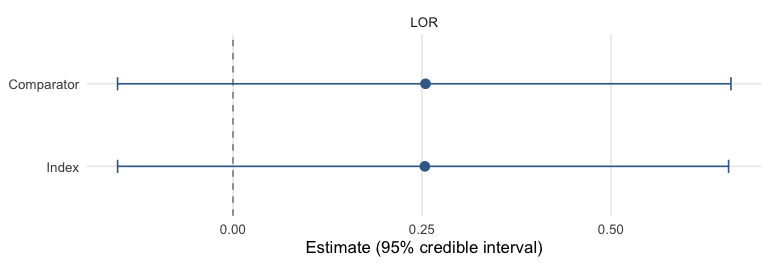

plot of chunk intervals

For convergence diagnostics on the raw draws, bayesplot needs to know which chain each draw came from. fit$draws is a flat data frame with the chains already stacked, so passing it directly draws one merged line per parameter. That looks like a healthy trace whatever the chains did, because the thing a trace plot exists to show, whether the chains agree with each other, has been averaged away before plotting. The per-draw chain labels are kept beside the draws in fit$chain_ids, so reshape into the iteration by chain by parameter array bayesplot expects:

pars <- c("lor_index", "lor_comparator")
chain <- fit$chain_ids
# NULL means the backend could not label the draws, which is itself worth
# knowing: without labels there is no chain comparison to draw.
stopifnot(!is.null(chain))

# `split()` keeps each chain's draws in iteration order, which is what a trace
# needs. Indexing by a chain's own label rather than by arithmetic on the row
# count avoids assuming the chains are equal length or stored in order.
rows_by_chain <- split(seq_along(chain), chain)
n_iter <- unique(lengths(rows_by_chain))
stopifnot(length(n_iter) == 1L)

draws_array <- array(
  NA_real_,
  dim = c(n_iter, length(rows_by_chain), length(pars)),
  dimnames = list(NULL, paste("chain", names(rows_by_chain)), pars)
)
for (k in seq_along(rows_by_chain)) {
  draws_array[, k, ] <- as.matrix(fit$draws[rows_by_chain[[k]], pars])
}

bayesplot::mcmc_trace(draws_array) +
  ggplot2::labs(title = "Trace plots")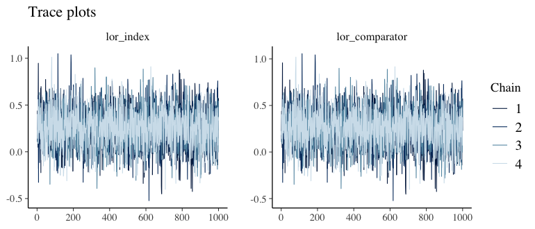

plot of chunk trace

Each chain is drawn separately, which is what makes the plot readable as a diagnostic: chains that settled in different places show up as separated bands. check_diagnostics() answers the same question numerically through split-Rhat and effective sample size, and the two should agree.

Prior sensitivity

prior_sensitivity() refits across a grid of prior_beta scales, holding every other model setting fixed, so any movement in the summaries is attributable to the prior alone. The fit used here is the SPFA model built above, where the coefficients are identified by the IPD and the sweep is expected to be flat:

prior_sensitivity(fit, prior_beta_scales = c(1, 2.5, 5))
#> Running MCMC with 4 parallel chains...
#> 
#> Chain 1 finished in 1.4 seconds.
#> Chain 2 finished in 1.3 seconds.
#> Chain 3 finished in 1.2 seconds.
#> Chain 4 finished in 1.3 seconds.
#> 
#> All 4 chains finished successfully.
#> Mean chain execution time: 1.3 seconds.
#> Total execution time: 1.6 seconds.
#> Running MCMC with 4 parallel chains...
#> 
#> Chain 1 finished in 1.6 seconds.
#> Chain 2 finished in 1.4 seconds.
#> Chain 3 finished in 1.4 seconds.
#> Chain 4 finished in 1.4 seconds.
#> 
#> All 4 chains finished successfully.
#> Mean chain execution time: 1.5 seconds.
#> Total execution time: 1.8 seconds.
#> Running MCMC with 4 parallel chains...
#> 
#> Chain 1 finished in 1.1 seconds.
#> Chain 4 finished in 1.0 seconds.
#> Chain 2 finished in 1.1 seconds.
#> Chain 3 finished in 1.1 seconds.
#> 
#> All 4 chains finished successfully.
#> Mean chain execution time: 1.1 seconds.
#> Total execution time: 1.3 seconds.
#> 
#> Prior sensitivity: posterior of marginal treatment effects
#> =========================================================
#> 
#>  scale      parameter effect      mean        sd       q2.5       q50     q97.5
#>    1.0      lor_index    LOR 0.2450842 0.2042432 -0.1572848 0.2449714 0.6380143
#>    1.0 lor_comparator    LOR 0.2459477 0.2050747 -0.1581046 0.2454590 0.6396459
#>    2.5      lor_index    LOR 0.2537767 0.2053081 -0.1526689 0.2538476 0.6555978
#>    2.5 lor_comparator    LOR 0.2546679 0.2061737 -0.1527328 0.2545148 0.6587242
#>    5.0      lor_index    LOR 0.2481648 0.2012573 -0.1446230 0.2465931 0.6394745
#>    5.0 lor_comparator    LOR 0.2490404 0.2020809 -0.1439587 0.2471842 0.6418033
#> 
#> Interpretation: approximately constant summaries show the posterior
#> is insensitive to the beta-prior SCALES tested here. That is not the
#> same as the inference being data-driven: identification also depends
#> on the prior family and location, the comparator-specific and
#> auxiliary priors, and the model structure. Vary those too. For a
#> non-survival fit, check_identification() adds the geometry of the
#> aggregate rows: exact for a normal identity-link model, descriptive
#> otherwise.

The case that motivates the check is the relaxed model, whose comparator coefficients are informed only through the aggregate likelihood and can therefore be prior-sensitive. For a relaxed binomial, normal, or poisson fit, run check_identification() on the data first, since a sweep cannot repair a design that carries no information about a coefficient, then pass the relaxed fit to prior_sensitivity() and sweep the comparator prior alongside the index one with prior_beta_comparator_scales. See vignette("subgroup-identification", "mlumr"). Survival is the exception: check_identification() refuses it, because a reconstructed comparator curve is not a set of scalar subgroup summaries and a row count neither bounds nor certifies what it identifies. For a relaxed survival fit, inspect the coefficient posterior and use the prior sweep. The reported marginal posterior-to-prior variance change is descriptive and is not a fraction learned from the data.

Troubleshooting

Divergent transitions, raise adapt_delta (e.g. 0.99).
Slow convergence / low ESS, increase iter and warmup.
Relaxed-model identifiability, with little AgD, the comparator-specific coefficients are weakly identified (mlumr warns). Use SPFA if effect modification is not expected, supply more informative prior_beta, or run prior_sensitivity().