Choosing a method for single-arm indirect comparisons: ML-UMR, STC, and naive • mlumr

library(mlumr)
library(ggplot2)
options(mc.cores = parallel::detectCores())

Every method in this vignette is a method for single-arm indirect comparisons: fully unanchored comparisons of fully disconnected evidence, where IPD for one treatment and AgD for the other share no common reference arm. If the evidence is connected through a common arm, none of them is the right tool; see the decision guide below. Single-arm indirect comparisons rest on strong, partly untestable assumptions, so running several methods and comparing them is itself a sensitivity analysis. mlumr offers four estimators for this setting behind one data interface; this vignette explains what each assumes, how to compare them, and which to report. For the mechanics of fitting see vignette("fitting-and-diagnostics"); for family-specific worked examples see the per-outcome vignettes. We illustrate with the real plaque-psoriasis binary endpoint (PASI 75; UNCOVER-2 ixekizumab vs FIXTURE secukinumab) (Griffiths et al. 2015; Langley et al. 2014).

Method	Adjustment	Framework	Key assumption	Target population
Naive	none	frequentist	populations exchangeable	none (unstandardized contrast)
STC	unanchored outcome regression (G-computation)	frequentist	correct, applicable IPD outcome model	comparator
ML-UMR SPFA	joint Bayesian model	Bayesian	shared prognostic effects (SPFA)	index and comparator
ML-UMR relaxed	joint Bayesian model	Bayesian	correct + identified treatment-specific effects	index and comparator

The naive estimate is an unadjusted contrast of two samples rather than an effect standardized to any population. stc() standardizes the index-treatment outcome to the comparator population and contrasts it with the observed comparator outcome there. It does not standardize either treatment to the index population. Treating that comparator-population effect as the index or decision target requires a separate effect-equality assumption (Phillippo et al. 2016; Chandler and Ishak 2026). ML-UMR explicitly standardizes both treatment models to each reported target. Its validity still depends on the fitted outcome model, overlap, and the stated cross-treatment assumptions.

A shared dataset

All four estimators run from the same mlumr_data object, so we build it once, the plaque-psoriasis PASI 75 endpoint (UNCOVER-2 ixekizumab vs FIXTURE secukinumab) with three prognostic covariates.

Hypothetical single-arm trials. UNCOVER-2 and FIXTURE are randomized trials. Dropping their common reference arms (placebo and etanercept) turns them into hypothetical single-arm trials and leaves fully disconnected evidence; we do this only to illustrate ML-UMR. In practice, randomized trials should never be analyzed this way: ML-NMR (for example with multinma) or another appropriate method should be used for them. ML-UMR should only be used for fully unanchored, single-arm comparisons.

The single-arm IPD and AgD for this comparison:

data("psoriasis_ipd")   # bundled with mlumr (from multinma, GPL-3)
data("psoriasis_agd")

covs <- c("age", "bsa", "weight")
ipd <- psoriasis_ipd
ipd$bsa <- ipd$bsa / 100; ipd$weight <- ipd$weight / 10
ipd <- ipd[ipd$study == "UNCOVER-2" & ipd$treatment == "IXE_Q4W", ]
ipd <- ipd[stats::complete.cases(ipd[, c("pasi75", covs)]), ]

agd <- psoriasis_agd
agd$bsa_mean <- agd$bsa_mean / 100; agd$bsa_sd <- agd$bsa_sd / 100
agd$weight_mean <- agd$weight_mean / 10; agd$weight_sd <- agd$weight_sd / 10
agd <- agd[agd$study == "FIXTURE" & agd$treatment == "SEC_300", ]

dat <- combine_data(
  set_ipd(ipd, treatment = "treatment", outcome = "pasi75", covariates = covs),
  set_agd(agd, treatment = "treatment", outcome_n = "pasi75_n", outcome_r = "pasi75_r",
          cov_means = c("age_mean", "bsa_mean", "weight_mean"),
          cov_sds   = c("age_sd", "bsa_sd", "weight_sd"),
          cov_types = c("continuous", "continuous", "continuous")))
# `bsa` was rescaled to a proportion above, so its marginal has to respect
# (0, 1). A normal marginal puts integration points outside that range;
# `vignette("binary-outcomes")` uses the logit-normal for the same reason.
dat <- add_integration(dat, n_int = 64,
  age    = distr(qnorm,      mean = age_mean, sd = age_sd),
  bsa    = distr(qlogitnorm, mean = bsa_mean, sd = bsa_sd),
  weight = distr(qgamma, shape = weight_mean^2 / weight_sd^2,
                 rate = weight_mean / weight_sd^2))

Naive and STC

The naive estimate compares crude outcomes with no covariate adjustment. It serves as a benchmark, and it is biased when the two studies differ on prognostic covariates or on other determinants of the outcome; a difference in the distribution of a variable unrelated to the outcome does not by itself induce bias. STC fits an outcome regression on the IPD and predicts outcomes under the index treatment in the comparator population by G-computation. The response-scale averaging follows Ren et al.’s unanchored single-arm STC and the marginalization order used by Remiro-Azocar et al. (Ren et al. 2024; Remiro-Azocar et al. 2022). The non-survival delta-method SE is conditional on the supplied integration grid and reported covariate summaries; it does not reproduce Ren et al.’s bootstrap of both the IPD fit and reconstructed target distribution.

res_naive <- naive(dat)
res_stc   <- stc(dat)
res_naive
#> Naive Unadjusted Indirect Comparison
#> =====================================
#> 
#> Treatments: IXE_Q4W vs SEC_300 
#> 
#> Population basis: index-study outcome versus comparator-population outcome; no common standardized target.
#> 
#> Event rates:
#>   Index (IPD):      0.774 (267/345)
#>   Comparator (AgD): 0.771 (249/323)
#> 
#> Log Odds Ratio: 0.0172 (SE: 0.1846)
#> 95% CI: [-0.3448, 0.3791]
#> 
#> All effect measures (95% CI):
#>   Log odds ratio                 0.0172 (SE 0.1846) [-0.3448, 0.3791]
#>   Odds ratio                     1.0173 [0.7084, 1.4609]
#>   Risk difference                0.0030 (SE 0.0325) [-0.0606, 0.0666]
#>   Risk ratio                     1.0039 [0.9245, 1.0901]
res_stc
#> Simulated Treatment Comparison (G-computation)
#> ===============================================
#> 
#> Treatments: IXE_Q4W vs SEC_300 
#> 
#> Estimand population: comparator
#> Treating this as the index-population effect requires a separate effect-equality assumption; this calculation does not transport to the index population.
#> 
#> Marginalized P(Y=1|index trt, comp pop): 0.8111
#> Observed P(Y=1|comp trt, comp pop):      0.7709
#> 
#> Log Odds Ratio: 0.2437 (SE: 0.2021)
#> 95% CI: [-0.1524, 0.6399]
#> 
#> All effect measures (95% CI):
#>   Log odds ratio                 0.2437 (SE 0.2021) [-0.1524, 0.6399]
#>   Odds ratio                     1.2760 [0.8586, 1.8962]
#>   Risk difference                0.0402 (SE 0.0331) [-0.0246, 0.1050]
#>   Risk ratio                     1.0521 [0.9693, 1.1421]
#> 
#> Outcome model coefficients:
#> (Intercept)         age         bsa      weight 
#>      4.4675     -0.0400      0.0848     -0.1430

ML-UMR (SPFA and relaxed)

The two Bayesian models share the same data interface and differ only in whether the prognostic coefficients are shared across treatments (SPFA) or allowed to be treatment-specific (relaxed, permitting effect modification):

fit_spfa <- mlumr(dat, model = "spfa",
                  prior_beta = prior_normal(0, 2.5, autoscale = TRUE),
                  chains = 4, iter = 2000, warmup = 1000, seed = 2026, refresh = 0)
#> Running MCMC with 4 parallel chains...
#> 
#> Chain 1 finished in 0.5 seconds.
#> Chain 2 finished in 0.5 seconds.
#> Chain 3 finished in 0.5 seconds.
#> Chain 4 finished in 0.5 seconds.
#> 
#> All 4 chains finished successfully.
#> Mean chain execution time: 0.5 seconds.
#> Total execution time: 0.8 seconds.
fit_relaxed <- mlumr(dat, model = "relaxed",
                     prior_beta = prior_normal(0, 2.5, autoscale = TRUE),
                     chains = 4, iter = 2000, warmup = 1000, seed = 2026, refresh = 0)
#> Running MCMC with 4 parallel chains...
#> 
#> Chain 1 finished in 2.4 seconds.
#> Chain 2 finished in 2.8 seconds.
#> Chain 4 finished in 2.7 seconds.
#> Chain 3 finished in 2.9 seconds.
#> 
#> All 4 chains finished successfully.
#> Mean chain execution time: 2.7 seconds.
#> Total execution time: 3.1 seconds.

A comparison table

All four single-arm methods, on the log odds ratio. ML-UMR is reported in both target populations. STC has a comparator-population estimand by construction; naive has no single standardized target and is labeled accordingly. Neither has an index-population row to show. Which of them is decision-relevant is a question about the application, not a property of the method: a cost-effectiveness model is built for the population the reimbursement decision covers, and that population has to be stated. It is often close to the index trial’s (Chandler and Ishak 2026), which is why the index row usually carries the decision, but it is not automatically either trial’s. When the decision population is a third one, standardize to it directly by passing its covariate distribution as newdata to predict() or marginal_effects(), which average over those rows, rather than adopting whichever trial is nearer. conditional_effects() takes the same data frame and evaluates at each profile separately rather than averaging over them, so what it returns is a set of conditional effects and not a transported marginal one. The comparator rows are the like-for-like comparison against STC, which standardizes to that population; naive standardizes to neither and is the unadjusted benchmark both rows are measured against.

me_spfa <- marginal_effects(fit_spfa, effect = "lor", population = "both")
me_rel  <- marginal_effects(fit_relaxed, effect = "lor", population = "both")
# One row per (model, population); `pop()` pulls the requested one.
pop <- function(d, which) d[d$population == which, ]
comparison <- data.frame(
  Method = c("Naive", "STC", "ML-UMR SPFA", "ML-UMR SPFA",
             "ML-UMR relaxed", "ML-UMR relaxed"),
  Population = c("unstandardized", "comparator", "index", "comparator",
                 "index", "comparator"),
  LOR      = c(res_naive$link_effect, res_stc$link_effect,
               pop(me_spfa, "Index")$mean, pop(me_spfa, "Comparator")$mean,
               pop(me_rel, "Index")$mean, pop(me_rel, "Comparator")$mean),
  CI_lower = c(res_naive$ci_lower, res_stc$ci_lower,
               pop(me_spfa, "Index")$q2.5, pop(me_spfa, "Comparator")$q2.5,
               pop(me_rel, "Index")$q2.5, pop(me_rel, "Comparator")$q2.5),
  CI_upper = c(res_naive$ci_upper, res_stc$ci_upper,
               pop(me_spfa, "Index")$q97.5, pop(me_spfa, "Comparator")$q97.5,
               pop(me_rel, "Index")$q97.5, pop(me_rel, "Comparator")$q97.5)
)
knitr::kable(comparison, caption = "PASI 75 log odds ratio by method, in both target populations")

PASI 75 log odds ratio by method, in both target populations
Method	Population	LOR	CI_lower	CI_upper
Naive	unstandardized	0.0171520	-0.3447542	0.3790582
STC	comparator	0.2437223	-0.1524312	0.6398759
ML-UMR SPFA	index	0.2442120	-0.1440524	0.6435369
ML-UMR SPFA	comparator	0.2459988	-0.1446246	0.6508805
ML-UMR relaxed	index	-0.0211377	-1.2249046	1.0791852
ML-UMR relaxed	comparator	0.2470542	-0.1473308	0.6289507

forest_df <- with(comparison,
  data.frame(label = paste0(Method, " (", Population, ")"),
             est = LOR, lo = CI_lower, hi = CI_upper))
mlumr_forest(forest_df, ref_line = 0,
             x = "Log odds ratio",
             title = "Methods compared: ixekizumab vs secukinumab",
             subtitle = "ML-UMR shown in both target populations")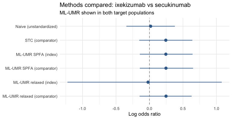

plot of chunk forest

The same ML-UMR posteriors straight from marginal_effects(), whose plot() method shows both populations by default:

plot(marginal_effects(fit_spfa, effect = "lor"))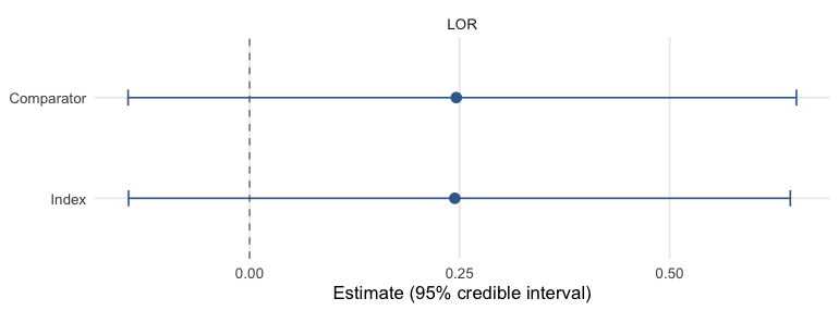

plot of chunk posterior-both

Interpreting the differences

Naive vs STC, the gap reflects the combined effects of standardization, outcome-model specification, and the different target definitions. Agreement does not establish exchangeability, and disagreement is not attributable to one covariate without further analysis.
STC vs ML-UMR SPFA, both use the named covariates, but they fit different likelihoods and make different cross-treatment assumptions. Similarity is a useful benchmark, not an expected mathematical identity. ML-UMR reports explicitly standardized effects in both populations.
SPFA vs relaxed, the relaxed model frees prognostic effects to differ by treatment (delta_beta); a markedly different effect may signal effect modification, but the comparator coefficients are weakly identified with sparse AgD, so check delta_beta and prior_sensitivity().
Index vs comparator within the relaxed model, note how much wider the index-population interval is than the comparator one in the table above. A single aggregate row constrains the comparator coefficients only through one combination with the comparator intercept, and the index-population estimand extrapolates them over the IPD covariate distribution, so the width is the identification problem showing itself. Under SPFA the two populations agree closely instead, because the coefficients are shared and anchored by the IPD.

Model comparison

Information criteria compare approximate predictive fit; they do not validate SPFA, effect modification, or transportability. We compare SPFA against the relaxed model by leave-one-out cross-validation and DIC:

compare_models(SPFA = fit_spfa, Relaxed = fit_relaxed, criterion = "loo")
#> 
#> Model Comparison (LOO)
#> ======================
#> 
#>    model elpd_diff se_diff p_worse       diag_diff      diag_elpd
#>  Relaxed       0.0     0.0      NA                 1 k_psis > 0.7
#>     SPFA      -0.2     0.1    0.99 |elpd_diff| < 4 1 k_psis > 0.7
#> 
#> 
#> elpd_diff is the difference in expected log pointwise predictive
#> density vs the best model, and se_diff is its standard error: the
#> uncertainty about that difference, not evidence for it. Read the two
#> together. A difference small relative to se_diff is not distinguished
#> from zero by this comparison, whatever se_diff itself is.
#> Treat any ratio as a heuristic, not a decision rule, and check the
#> PSIS diagnostics and whether the difference matters for the
#> prediction you care about.
compare_models(SPFA = fit_spfa, Relaxed = fit_relaxed)   # DIC-based (the default)
#> 
#> Model Comparison (DIC)
#> ======================
#> 
#>    Model    DIC   pD Delta_DIC
#>  Relaxed 366.10 4.84      0.00
#>     SPFA 366.17 4.74      0.07
#> 
#> Lower DIC = better fit. Delta_DIC > 5 is a rough heuristic for
#> meaningful difference, not a formally calibrated threshold.
#> DIC should not be the sole basis for model selection.

LOO/WAIC are preferred over DIC where available; treat a better-fitting relaxed model as suggestive of effect modification, not proof, corroborate with delta_beta, prior sensitivity, and clinical plausibility. Treat these as approximate fit diagnostics rather than exact predictive scores: each aggregate-data row enters the pointwise log-likelihood as a single independent observation, so LOO/WAIC do not reflect the grouped (study-level) structure of the comparator evidence and can be optimistic when the AgD is clustered.

Decision guide

Is there a common comparator arm? If the two trials share an arm, run an anchored analysis instead: a network meta-analysis, or ML-NMR via multinma when the populations differ. Randomization is doing work there that nothing below replaces, so trials connected through a common arm should never be broken into single-arm evidence. Reserve ML-UMR, and every method in this vignette, for single-arm indirect comparisons of fully disconnected evidence. vignette("binary-outcomes") and vignette("survival-outcomes") each end by restoring the common arm their example discards and checking the unanchored answer against two anchored ones, a Bucher indirect comparison and an ML-NMR fitted with multinma, each in both a prognostic-only and a treatment-interaction form.
Are the two populations exchangeable on prognostic factors? Similar reported marginal means are weak evidence for this: higher moments, the dependence between covariates, and unreported prognostic variables all matter, and none is visible in a baseline table. Treat the naive estimate as a benchmark rather than a candidate primary analysis unless exchangeability is defensible on substantive grounds.
Is the SPFA plausible? If it is the prespecified scientific assumption, ML-UMR SPFA can be the primary analysis and the relaxed model can probe that assumption. If uncertain, fit both. Before reading anything into a disagreement, check that the relaxed model is identified, with check_identification() on the data (binomial, normal, and poisson; it refuses survival, where a reconstructed curve is not a scalar subgroup summary) and prior_sensitivity() on the fit. Where the aggregate evidence is weak, a divergence between the two is evidence about identification, not about effect modification, and the relaxed index-population estimate belongs in a sensitivity analysis.
Presentation. Choose the estimator that is scientifically defensible first, then adapt how it is presented. Where a frequentist summary is expected, STC can be reported alongside ML-UMR rather than in place of it.

Always report the naive estimate as a benchmark, and report ML-UMR diagnostics (divergences, Rhat, ESS) alongside the estimates.

References

Chandler, Conor, and K. Jack Ishak. 2026. Reframing Population-Adjusted Indirect Comparisons as a Transportability Problem: An Estimand-Based Perspective and Implications for Health Technology Assessment. Preprint. https://doi.org/10.48550/arXiv.2602.17041.

Griffiths, C. E. M., K. Reich, M. Lebwohl, et al. 2015. “Comparison of Ixekizumab with Etanercept or Placebo in Moderate-to-Severe Psoriasis (UNCOVER-2 and UNCOVER-3): Results from Two Phase 3 Randomised Trials.” The Lancet 386 (9993): 541–51. https://doi.org/10.1016/s0140-6736(15)60125-8.

Langley, R. G., B. E. Elewski, M. Lebwohl, et al. 2014. “Secukinumab in Plaque Psoriasis — Results of Two Phase 3 Trials.” New England Journal of Medicine 371 (4): 326–38. https://doi.org/10.1056/nejmoa1314258.

Phillippo, D. M., A. E. Ades, S. Dias, S. Palmer, K. R. Abrams, and N. J. Welton. 2016. NICE DSU Technical Support Document 18: Methods for Population-Adjusted Indirect Comparisons in Submissions to NICE. National Institute for Health and Care Excellence Decision Support Unit. https://www.sheffield.ac.uk/nice-dsu/tsds/population-adjusted.

Remiro-Azocar, Antonio, Anna Heath, and Gianluca Baio. 2022. “Parametric g-Computation for Compatible Indirect Treatment Comparisons with Limited Individual Patient Data.” Research Synthesis Methods 13 (6): 716–44. https://doi.org/10.1002/jrsm.1565.

Ren, Shijie, Sa Ren, Nicky J. Welton, and Mark Strong. 2024. “Advancing Unanchored Simulated Treatment Comparisons: A Novel Implementation and Simulation Study.” Research Synthesis Methods 15 (4): 657–70. https://doi.org/10.1002/jrsm.1718.