Preparing data and integration points • mlumr

Every mlumr analysis follows the same four-step pipeline. This vignette covers the family-agnostic machinery, combining IPD and AgD and, above all, the numerical integration that powers population adjustment. The exact set_ipd() / set_agd() arguments for each outcome family are shown, with complete runnable examples, in the per-outcome vignettes (see the reference table below).

set_ipd(), individual patient data (the index treatment)
set_agd() (or set_agd_surv() for survival), aggregate data (comparator)
combine_data(), join them into one mlumr_data object
add_integration(), quasi-Monte Carlo integration points (ML-UMR only)

The pipeline (illustrated on a binary endpoint)

The four steps below build a complete mlumr_data object from a binary IPD trial and a one-row aggregate comparator; the sections that follow explain each piece (covariate naming, integration, correlation) in detail:

library(mlumr)
set.seed(2026)

# IPD (index): one row per patient
trial_a <- data.frame(
  treatment = "Drug_A",
  response = rbinom(500, 1, 0.6),
  age_group = rbinom(500, 1, 0.4),
  sex = rbinom(500, 1, 0.55)
)
ipd <- set_ipd(trial_a, treatment = "treatment", outcome = "response",
               covariates = c("age_group", "sex"))

# AgD (comparator): one row per study, with covariate summaries
trial_b <- data.frame(
  treatment = "Drug_B", n_total = 400, n_events = 160,
  age_group_mean = 0.35, sex_prop = 0.50
)
agd <- set_agd(trial_b, treatment = "treatment",
               outcome_n = "n_total", outcome_r = "n_events",
               cov_means = c("age_group_mean", "sex_prop"),
               cov_types = c("binary", "binary"))

dat <- combine_data(ipd, agd)
dat
#> Unanchored Comparison Data (Binary)
#> ====================================
#> 
#> Index treatment (IPD): Drug_A 
#>   N = 500 
#>   Events = 303 (60.6%) 
#> 
#> Comparator treatment (AgD): Drug_B 
#>   N = 400 
#>   Events = 160 (40.0%) 
#> 
#> Covariates ( 2 ): age_group, sex 
#> Integration points: not yet added (use add_integration())

Outcome-family input reference

The outcome arguments differ by family; everything else (covariates, combining, integration) is identical. Each family has a complete worked example.

Family	`set_ipd()` outcome args	`set_agd()` outcome args	Vignette
binomial	`outcome` (0/1)	`outcome_n`, `outcome_r`	`vignette("binary-outcomes")`
normal	`outcome`, `family = "normal"`	`outcome_mean`, `outcome_se` (+ `outcome_n`)	`vignette("continuous-outcomes")`
poisson	`outcome`, `exposure`, `family = "poisson"`	`outcome_r`, `outcome_E`	`vignette("count-outcomes")`
survival	`Surv`/`time`/`status`, `family = "survival"`	`set_agd_surv()`: pseudo-IPD `time`/`status`	`vignette("survival-outcomes")`

set_ipd() validates that the outcome matches the family (binary 0/1; numeric for normal; non-negative integer counts for Poisson; positive times for survival) and drops rows with missing values (with a warning).

Covariate naming and types

set_agd() strips _mean and _prop suffixes so AgD covariate names match the IPD (age_group_mean → age_group, sex_prop → sex). Declare each covariate as "binary" or "continuous" via cov_types; continuous covariates also need a standard-deviation column in cov_sds.

Scale conventions for aggregate summaries

For the normal family, outcome_mean and outcome_se must be on the original (arithmetic) scale, the same scale as the IPD outcome, even when fitting with link = "log". A geometric mean will not do, and its units are what makes that easy to miss: it is in the original units and is still a different quantity. Exponentiating a log-scale mean gives the geometric mean, not the arithmetic one, and for a lognormal outcome with log-scale SD 1 the geometric mean is 39% below the arithmetic one, which is the same gap seen from the other side as the arithmetic mean being 65% above it. Propagating the standard error does not repair that, because the mismatch is in the estimand rather than in its uncertainty. Ask for the arithmetic mean and its SE. See vignette("continuous-outcomes").

Integration points

ML-UMR adjusts for covariate imbalance by integrating the IPD-derived outcome model over the comparator population’s covariate distribution. mlumr represents that distribution by Sobol quasi-Monte Carlo (QMC) integration points, correlated with a Gaussian copula so the joint covariate structure is respected.

dat <- add_integration(
  dat,
  n_int = 64,
  age_group = distr(qbern, prob = age_group_mean),
  sex = distr(qbern, prob = sex_mean)
)

n_int, number of points (powers of 2: 32, 64, 128, …). More points give better accuracy at the cost of slower fitting; check adequacy with check_integration() (below).
distr(), wraps a quantile function whose parameters reference AgD summary columns. Use qbern (Bernoulli, supplied by mlumr) for binary covariates, qnorm for normal, qgamma for skewed positive covariates, and qlogitnorm for a covariate reported as a proportion on (0, 1).

mlumr’s qgamma() and qlogitnorm() accept a mean and sd on the natural scale in place of their native parameters, so the moments can be taken from a published baseline table without conversion. Both must be supplied together. A logit-normal additionally requires sd^2 < mean * (1 - mean), the bound any variable on (0, 1) satisfies; a percentage must be rescaled to a proportion first.

add_integration(
  dat, n_int = 64,
  age = distr(qbern, prob = age_mean),                  # binary
  bmi = distr(qnorm, mean = bmi_mean, sd = bmi_sd),     # continuous (normal)
  biomarker = distr(qgamma, mean = bio_mean, sd = bio_sd),  # right-skewed
  bsa = distr(qlogitnorm, mean = bsa_mean, sd = bsa_sd)     # proportion on (0, 1)
)

Correlation handling

By default the covariate correlation is estimated from the IPD (Spearman) and adjusted for the Gaussian copula. For binary and mixed discrete/continuous pairs this copula adjustment is a pragmatic approximation: the exact latent Gaussian correlation depends on the marginal prevalences, which the current transform does not use. It is adequate for most datasets, but if you have strong prior information, or covariates with prevalences near 0/1, strong correlations, or many covariates, supply your own matrix via cor and confirm the result is stable with check_integration().

my_cor <- matrix(c(1, 0.3, 0.3, 1), 2, 2)
add_integration(dat, n_int = 64, cor = my_cor,
                age_group = distr(qbern, prob = age_group_mean),
                sex = distr(qbern, prob = sex_mean))

add_integration(dat, n_int = 64, cor_adjust = "none",  # no adjustment
                age_group = distr(qbern, prob = age_group_mean),
                sex = distr(qbern, prob = sex_mean))

Inspecting the integration points

unnest_integration() expands the stored points to a data frame with one row per aggregate row and integration point, one column per covariate, plus .int_id and .agd_row, so you can inspect or plot the realized comparator distribution directly:

head(unnest_integration(dat))     # one row per point, covariates in columns
#>   age_group sex .int_id .agd_row
#> 1         0   0       1        1
#> 2         1   0       2        1
#> 3         0   1       3        1
#> 4         0   0       4        1
#> 5         1   1       5        1
#> 6         0   0       6        1

check_integration(
  dat,
  age_group = distr(qbern, prob = age_group_mean),
  sex = distr(qbern, prob = sex_mean)
)
#> Integration check: n_int = 64 vs 128
#> Resolution heuristic, max relative difference: 0.0079
#> Resolution stable within the package's 1% heuristic.
#> Declared-target fidelity, max relative difference: 0.0156
#> Caution: grid moments differ from declared AgD moments by 1-5%.
#> Joint: max |cor(current) - cor(doubled)|: 0.0113
#> Joint resolution stable within the package's 0.05 heuristic.
#> Target (spearman): max |cor(doubled) - cor_target|: 0.0196

check_integration() compares the realized integration points against the requested marginals and correlations and flags when n_int is too small, run it whenever there are several or strongly correlated covariates.

Visualizing the integration points

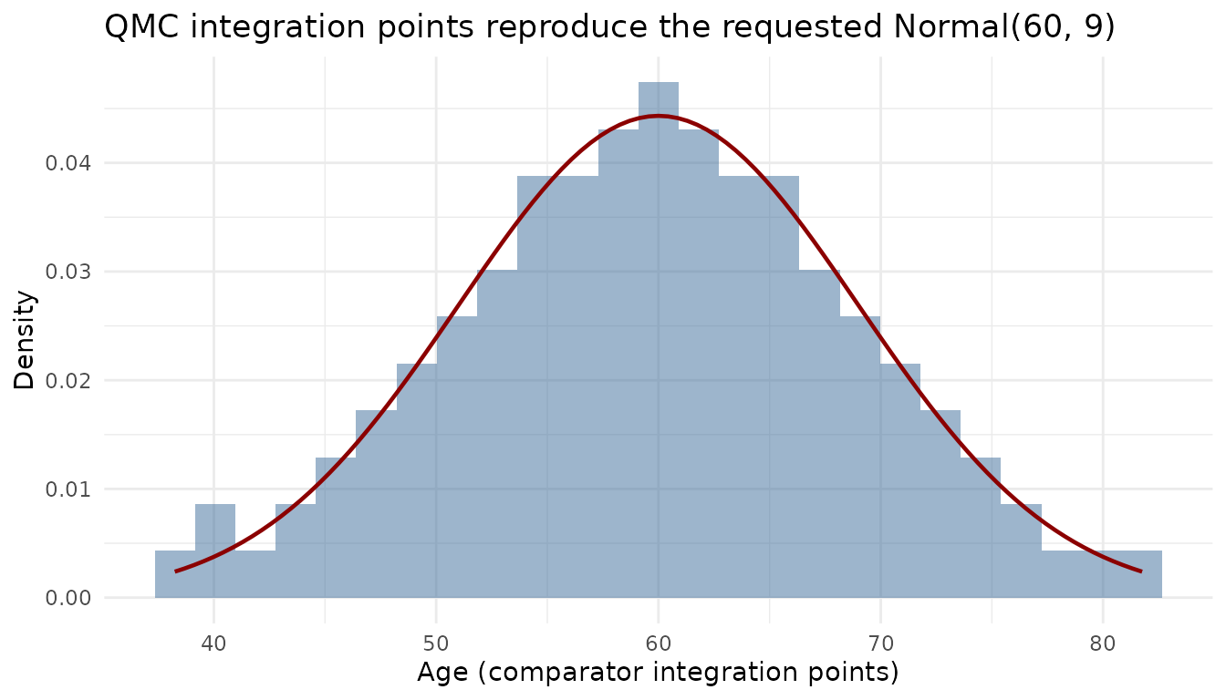
For a continuous covariate the quasi-Monte Carlo points should reproduce the requested marginal. Here we build a small example with a continuous age and overlay the integration points on the requested Normal density:

set.seed(2026)
ipd_c <- data.frame(treatment = "Drug_A", response = rbinom(400, 1, 0.5),
                    age = rnorm(400, 55, 10))
agd_c <- data.frame(treatment = "Drug_B", n_total = 300, n_events = 120,
                    age_mean = 60, age_sd = 9)
dat_c <- combine_data(
  set_ipd(ipd_c, treatment = "treatment", outcome = "response", covariates = "age"),
  set_agd(agd_c, treatment = "treatment", outcome_n = "n_total",
          outcome_r = "n_events", cov_means = "age_mean", cov_sds = "age_sd",
          cov_types = "continuous"))
dat_c <- add_integration(dat_c, n_int = 128,
                         age = distr(qnorm, mean = age_mean, sd = age_sd))
pts <- unnest_integration(dat_c)

if (requireNamespace("ggplot2", quietly = TRUE)) {
  library(ggplot2)
  ggplot(pts, aes(age)) +
    geom_histogram(aes(y = after_stat(density)), bins = 25,
                   fill = "#3B6B9A", alpha = 0.5) +
    stat_function(fun = dnorm, args = list(mean = 60, sd = 9),
                  color = "darkred", linewidth = 0.8) +
    labs(x = "Age (comparator integration points)", y = "Density",
         title = "QMC integration points reproduce the requested Normal(60, 9)") +
    theme_minimal()
}

Integration requirements for STC and naive

naive() can be called immediately after combine_data() because it uses only the observed crude outcomes. stc() requires integration points for nonlinear links, including binomial and Poisson outcomes and normal-log models. Replacing a covariate distribution by its mean before applying a nonlinear inverse link does not recover the marginal outcome. Only the normal identity-link STC can use the aggregate means directly; see vignette("choosing-a-method").

dat_no_int <- combine_data(ipd, agd)
naive(dat_no_int)
#> Naive Unadjusted Indirect Comparison
#> =====================================
#> 
#> Treatments: Drug_A vs Drug_B 
#> 
#> Population basis: index-study outcome versus comparator-population outcome; no common standardized target.
#> 
#> Event rates:
#>   Index (IPD):      0.606 (303/500)
#>   Comparator (AgD): 0.400 (160/400)
#> 
#> Log Odds Ratio: 0.8360 (SE: 0.1371)
#> 95% CI: [0.5673, 1.1047]
#> 
#> All effect measures (95% CI):
#>   Log odds ratio                 0.8360 (SE 0.1371) [0.5673, 1.1047]
#>   Odds ratio                     2.3071 [1.7635, 3.0183]
#>   Risk difference                0.2060 (SE 0.0328) [0.1417, 0.2703]
#>   Risk ratio                     1.5150 [1.3180, 1.7414]
stc(dat)
#> Simulated Treatment Comparison (G-computation)
#> ===============================================
#> 
#> Treatments: Drug_A vs Drug_B 
#> 
#> Estimand population: comparator
#> Treating this as the index-population effect requires a separate effect-equality assumption; this calculation does not transport to the index population.
#> 
#> Marginalized P(Y=1|index trt, comp pop): 0.6025
#> Observed P(Y=1|comp trt, comp pop):      0.4000
#> 
#> Log Odds Ratio: 0.8213 (SE: 0.1383)
#> 95% CI: [0.5503, 1.0923]
#> 
#> All effect measures (95% CI):
#>   Log odds ratio                 0.8213 (SE 0.1383) [0.5503, 1.0923]
#>   Odds ratio                     2.2736 [1.7339, 2.9812]
#>   Risk difference                0.2025 (SE 0.0332) [0.1375, 0.2675]
#>   Risk ratio                     1.5062 [1.3091, 1.7331]
#> 
#> Outcome model coefficients:
#> (Intercept)   age_group         sex 
#>      0.3515      0.1693      0.0142