
Binary outcomes: an unanchored PASI 75 comparison
Source:vignettes/binary-outcomes.Rmd
binary-outcomes.RmdThis vignette is a complete worked example of an
unanchored indirect comparison for a
binary endpoint, using plaque-psoriasis trial data
bundled with mlumr (psoriasis_ipd /
psoriasis_agd, copied from the GPL-3 multinma
package (Phillippo
2024)). It is the unanchored, two-study analogue of
multinma’s plaque_psoriasis ML-NMR example (Phillippo et al.
2020). For the shared data-preparation machinery see
vignette("data-preparation"); for sampler/prior/diagnostic
detail see vignette("fitting-and-diagnostics"); for how to
choose between methods see
vignette("choosing-a-method").
About these data.
psoriasis_ipd/psoriasis_agdare copied verbatim frommultinma; they were not re-simulated for mlumr. multinma’s patient records are themselves simulated to resemble the published UNCOVER-2 (Griffiths et al. 2015) and FIXTURE (Langley et al. 2014) trials. mlumr bundles one arm from each trial: ixekizumab Q4W from UNCOVER-2 and secukinumab 300 mg from FIXTURE. Both trials also randomized patients to placebo and etanercept, and those arms are deliberately omitted here. Keeping them would connect the two trials through a common comparator and make an anchored comparison possible, which is not the problem this vignette is about. The unanchored framing is a construction for illustration; the section Checking against the anchored comparison below puts the omitted arms back to use.Hypothetical single-arm trials. UNCOVER-2 and FIXTURE are randomized trials. Dropping their common reference arms (placebo and etanercept) turns them into hypothetical single-arm trials and leaves fully disconnected evidence; we do this only to illustrate ML-UMR. In practice, randomized trials should never be analyzed this way: ML-NMR (for example with
multinma) or another appropriate method should be used for them. ML-UMR should only be used for fully unanchored, single-arm comparisons.
The clinical question
We want the relative efficacy of two interleukin inhibitors on PASI 75 response (≥ 75% improvement in the Psoriasis Area and Severity Index) at week 12, when:
-
Index (IPD). We hold individual patient data for
ixekizumab Q4W (
IXE_Q4W) from the UNCOVER-2 trial (Griffiths et al. 2015). -
Comparator (AgD). Only published aggregate data are
available for secukinumab 300 mg (
SEC_300) from the FIXTURE trial (Langley et al. 2014).
The two trials share no common arm, so the comparison is
unanchored and relies on the shared-effect-modifier /
conditional-constancy assumptions discussed in
vignette("introduction"). ML-UMR adjusts for cross-trial
differences in prognostic factors by standardizing the IPD model to the
comparator population (and vice versa).
The ML-UMR model
On the index IPD, ML-UMR fits an individual-level logistic regression for the probability of PASI 75 response, \operatorname{logit}\Pr(y_{ik}=1\mid x_i)=\mu_k+x_i^\top\beta_k, where \mu_k is a treatment-specific intercept and \beta_k the vector of prognostic-factor coefficients. The aggregate comparator does not contribute patient rows; instead its likelihood is the individual model integrated over the comparator covariate distribution f_{\text{AgD}}(x) implied by the published moments, \bar p_k=\Pr(Y=1\mid \text{AgD population})=\int\operatorname{logit}^{-1}(\mu_k+x^\top\beta_k)\,f_{\text{AgD}}(x)\,dx, which mlumr approximates with quasi-Monte Carlo integration points (see Setting up the ML-UMR data). This is the same population-adjustment device as ML-NMR (Phillippo et al. 2020), specialized to the unanchored two-study case.
Two variants differ only in how the prognostic effects are shared across treatments:
- SPFA (shared prognostic factors) assumes \beta_{\text{index}}=\beta_{\text{comparator}}=\beta, the conditional-constancy / shared-effect-modifier assumption.
- Relaxed frees them, \beta_{\text{index}}\neq\beta_{\text{comparator}}, allowing effect modification at the cost of identifiability (the comparator coefficients are informed only by the single AgD likelihood term).
Population-standardized treatment effects are formed by averaging the \operatorname{logit}^{-1} predictions over a target population and contrasting the treatments, yielding effects in both the index and comparator populations.
SPFA is the unanchored analogue of the shared-effect-modifier assumption used in anchored comparisons, but it is a stronger assumption, so transportability is correspondingly harder to justify (Chandler and Ishak 2025). A useful consequence, reported from simulation (Chandler and Ishak 2025): in the scenarios that study examined, the comparator-population effect was recovered with little bias even when SPFA was violated, because the prognostic coefficients are anchored by the index IPD, whereas the index-population effect was biased when SPFA was wrongly imposed under strong effect modification. Read that as evidence from the data-generating mechanisms, effect sizes and sample sizes that were simulated, not as a guarantee that the comparator-population estimand tolerates any violation. (Restricted to the comparator population, the SPFA estimand has the same standardization target as unanchored STC. The estimators still differ: ML-UMR fits a joint likelihood in which the aggregate outcome informs the comparator intercept, whereas STC regresses on the IPD alone.)
# IPD + AgD bundled with mlumr (copied from multinma's plaque_psoriasis, GPL-3).
data("psoriasis_ipd")
data("psoriasis_agd")

covs <- c("age", "bsa", "weight", "prevsys")   # adjustment set for this example

# --- Index IPD: UNCOVER-2, ixekizumab Q4W -----------------------------------
ipd <- psoriasis_ipd
ipd$bsa     <- ipd$bsa / 100      # body-surface area: % -> proportion
ipd <- ipd[ipd$study == "UNCOVER-2" & ipd$treatment == "IXE_Q4W", ]
ipd <- ipd[stats::complete.cases(ipd[, c("pasi75", covs)]), ]

# --- Comparator AgD: FIXTURE, secukinumab 300 mg ----------------------------
agd <- psoriasis_agd
agd$bsa_mean    <- agd$bsa_mean / 100
agd$bsa_sd      <- agd$bsa_sd / 100
agd <- agd[agd$study == "FIXTURE" & agd$treatment == "SEC_300", ]
A glimpse of the individual patient data (one row per patient) and the single aggregate comparator row:
knitr::kable(head(ipd[, c("study", "treatment", "pasi75", covs)]),
caption = "Index IPD (UNCOVER-2, ixekizumab Q4W), first rows")| study | treatment | pasi75 | age | bsa | weight | prevsys |
|---|---|---|---|---|---|---|
| UNCOVER-2 | IXE_Q4W | 1 | 49 | 0.25 | 88.7 | 1 |
| UNCOVER-2 | IXE_Q4W | 1 | 33 | 0.29 | 96.3 | 1 |
| UNCOVER-2 | IXE_Q4W | 1 | 25 | 0.40 | 93.6 | 1 |
| UNCOVER-2 | IXE_Q4W | 0 | 60 | 0.20 | 112.0 | 1 |
| UNCOVER-2 | IXE_Q4W | 1 | 49 | 0.20 | 119.3 | 0 |
| UNCOVER-2 | IXE_Q4W | 1 | 58 | 0.16 | 92.0 | 1 |
knitr::kable(agd[, c("study", "treatment", "pasi75_r", "pasi75_n",
           "age_mean", "bsa_mean", "weight_mean", "prevsys_prop")],
caption = "Comparator AgD (FIXTURE, secukinumab 300 mg)")| study | treatment | pasi75_r | pasi75_n | age_mean | bsa_mean | weight_mean | prevsys_prop |
|---|---|---|---|---|---|---|---|
| FIXTURE | SEC_300 | 249 | 323 | 44.5 | 0.343 | 83 | 0.63 |
Covariate balance
Population adjustment is motivated by the fact that the two trial populations differ on prognostic factors. Comparing the index sample means against the published comparator means shows the imbalance we must adjust for:
balance <- data.frame(
  Covariate  = c("Age (years)", "Body-surface area (prop.)",
                 "Weight (kg)", "Previous systemic (prop.)"),
  Index_IXE  = c(mean(ipd$age), mean(ipd$bsa), mean(ipd$weight), mean(ipd$prevsys)),
  Comparator_SEC = c(agd$age_mean, agd$bsa_mean, agd$weight_mean, agd$prevsys_prop)
)
knitr::kable(balance, caption = "Prognostic-factor balance: index vs comparator population")| Covariate | Index_IXE | Comparator_SEC |
|---|---|---|
| Age (years) | 45.7275362 | 44.500 |
| Body-surface area (prop.) | 0.2761159 | 0.343 |
| Weight (kg) | 94.0605797 | 83.000 |
| Previous systemic (prop.) | 0.6782609 | 0.630 |
Setting up the ML-UMR data
set_ipd() takes the patient-level data;
set_agd() takes the comparator event count
(outcome_r), sample size (outcome_n), and
covariate summaries. Covariate column suffixes (_mean,
_sd) are stripped to match the IPD names.
ipd_obj <- set_ipd(ipd, treatment = "treatment", outcome = "pasi75", covariates = covs)

agd_obj <- set_agd(agd, treatment = "treatment",
                   outcome_n = "pasi75_n", outcome_r = "pasi75_r",
                   cov_means = c("age_mean", "bsa_mean", "weight_mean", "prevsys_prop"),
                   cov_sds   = c("age_sd", "bsa_sd", "weight_sd", NA),
                   cov_types = c("continuous", "continuous", "continuous", "binary"))

dat <- combine_data(ipd_obj, agd_obj)
dat
#> Unanchored Comparison Data (Binary)
#> ====================================
#>
#> Index treatment (IPD): IXE_Q4W
#>   N = 345
#>   Events = 267 (77.4%)
#>
#> Comparator treatment (AgD): SEC_300
#>   N = 323
#>   Events = 249 (77.1%)
#>
#> Covariates ( 4 ): age, bsa, weight, prevsys
#> Integration points: not yet added (use add_integration())
The comparator covariate distribution is represented by quasi-Monte
Carlo integration points drawn from each covariate’s marginal,
correlated via a Gaussian copula calibrated from the IPD. The marginals
are the ones multinma’s own plaque-psoriasis example uses: gammas for
the right-skewed age and weight, a logit-normal for body-surface area (a
proportion, so it must stay inside (0, 1)), and a Bernoulli
for previous systemic therapy. We use a modest n_int = 64
here so the vignette builds quickly; a real analysis would use several
hundred or more (see vignette("data-preparation")).
dat <- add_integration(
  dat, n_int = 64,
  # Marginals follow multinma's own plaque-psoriasis example: gamma for the
  # right-skewed continuous covariates, logit-normal for body surface area
  # (a proportion), Bernoulli for the binary one. mlumr's qgamma() and
  # qlogitnorm() accept a mean and sd directly, so the published baseline
  # table can be used as printed.
  age     = distr(qgamma,     mean = age_mean,    sd = age_sd),
  bsa     = distr(qlogitnorm, mean = bsa_mean,    sd = bsa_sd),
  weight  = distr(qgamma,     mean = weight_mean, sd = weight_sd),
  prevsys = distr(qbern,      prob = prevsys_mean)
)
check_integration() confirms the quasi-Monte Carlo
points reproduce the requested covariate moments, run it whenever
covariates are correlated or n_int is small:
check_integration(
  dat,
  age     = distr(qgamma,     mean = age_mean,    sd = age_sd),
  bsa     = distr(qlogitnorm, mean = bsa_mean,    sd = bsa_sd),
  weight  = distr(qgamma,     mean = weight_mean, sd = weight_sd),
  prevsys = distr(qbern,      prob = prevsys_mean)
)
#> Integration check: n_int = 64 vs 128
#> Resolution heuristic, max relative difference: 0.0310
#> Caution: 1-5% marginal relative difference. Consider increasing n_int.
#> Declared-target fidelity, max relative difference: 0.0638
#> Warning: grid moments differ from declared AgD moments by >5%.
#> Joint: max |cor(current) - cor(doubled)|: 0.1025
#> Warning: pairwise correlations differ by > 0.05 between resolutions.
#> Target (spearman): max |cor(doubled) - cor_target|: 0.0390
Frequentist benchmarks
The unadjusted (naive) comparison ignores the covariate imbalance; STC adjusts for it by parametric G-computation. Both are fast and serve as reference points.
res_naive <- naive(dat)
res_stc   <- stc(dat)
res_naive
#> Naive Unadjusted Indirect Comparison
#> =====================================
#>
#> Treatments: IXE_Q4W vs SEC_300
#>
#> Population basis: index-study outcome versus comparator-population outcome; no common standardized target.
#>
#> Event rates:
#>   Index (IPD):      0.774 (267/345)
#>   Comparator (AgD): 0.771 (249/323)
#>
#> Log Odds Ratio: 0.0172 (SE: 0.1846)
#> 95% CI: [-0.3448, 0.3791]
#>
#> All effect measures (95% CI):
#>   Log odds ratio                 0.0172 (SE 0.1846) [-0.3448, 0.3791]
#>   Odds ratio                     1.0173 [0.7084, 1.4609]
#>   Risk difference                0.0030 (SE 0.0325) [-0.0606, 0.0666]
#>   Risk ratio                     1.0039 [0.9245, 1.0901]
res_stc
#> Simulated Treatment Comparison (G-computation)
#> ===============================================
#>
#> Treatments: IXE_Q4W vs SEC_300
#>
#> Estimand population: comparator
#> Treating this as the index-population effect requires a separate effect-equality assumption; this calculation does not transport to the index population.
#>
#> Marginalized P(Y=1|index trt, comp pop): 0.8106
#> Observed P(Y=1|comp trt, comp pop):      0.7709
#>
#> Log Odds Ratio: 0.2403 (SE: 0.2029)
#> 95% CI: [-0.1575, 0.6380]
#>
#> All effect measures (95% CI):
#>   Log odds ratio                 0.2403 (SE 0.2029) [-0.1575, 0.6380]
#>   Odds ratio                     1.2716 [0.8543, 1.8928]
#>   Risk difference                0.0397 (SE 0.0332) [-0.0255, 0.1048]
#>   Risk ratio                     1.0515 [0.9683, 1.1418]
#>
#> Outcome model coefficients:
#> (Intercept)         age         bsa      weight     prevsys
#>      4.3879     -0.0404      0.0676     -0.0139      0.1003
Fitting the ML-UMR models
The binomial family supports "logit" (default),
"probit", and "cloglog" links. We fit both the
shared-prognostic-factor model (SPFA) and the
relaxed model (treatment-specific prognostic effects,
allowing effect modification). Because age is on a ~50-unit scale,
autoscale = TRUE keeps the coefficient prior’s contribution
on a common SD scale. The numerical scale is still an
application-specific choice and should be checked predictively.
fit_spfa <- mlumr(dat, model = "spfa", link = "logit",
                  prior_beta = prior_normal(0, 2.5, autoscale = TRUE),
                  chains = 4, iter = 2000, warmup = 1000,
                  seed = 2026, refresh = 0)
#> Running MCMC with 4 parallel chains...
#>
#> Chain 1 finished in 0.8 seconds.
#> Chain 2 finished in 0.8 seconds.
#> Chain 3 finished in 0.8 seconds.
#> Chain 4 finished in 0.8 seconds.
#>
#> All 4 chains finished successfully.
#> Mean chain execution time: 0.8 seconds.
#> Total execution time: 1.0 seconds.

fit_relaxed <- mlumr(dat, model = "relaxed", link = "logit",
                     prior_beta = prior_normal(0, 2.5, autoscale = TRUE),
                     chains = 4, iter = 2000, warmup = 1000,
                     seed = 2026, refresh = 0)
#> Running MCMC with 4 parallel chains...
#>
#> Chain 2 finished in 4.3 seconds.
#> Chain 4 finished in 4.7 seconds.
#> Chain 3 finished in 5.3 seconds.
#> Chain 1 finished in 5.7 seconds.
#>
#> All 4 chains finished successfully.
#> Mean chain execution time: 5.0 seconds.
#> Total execution time: 5.8 seconds.

summary(fit_spfa)
#> ML-UMR Model Summary
#> ====================
#>
#> Model: SPFA
#> Family: Binary
#> Link: logit
#> Engine: cmdstanr
#> Treatments: IXE_Q4W (IPD) vs SEC_300 (AgD)
#>
#> MCMC Diagnostics:
#>   Divergent transitions: 0
#>   Max treedepth hits: 0
#>   Max Rhat: 1.003
#>   Min ESS: 1836
#>
#> Intercepts (logit scale):
#>       variable     mean        sd      2.5%    97.5%     Rhat
#>       mu_index 1.433550 0.1566491 1.1431922 1.745167 1.002008
#>  mu_comparator 1.182341 0.1504401 0.8824316 1.474706 1.000581
#>
#> Regression Coefficients:
#>       variable        mean          sd        2.5%        97.5%     Rhat
#>      beta[age] -0.04089938 0.011061348 -0.06207939 -0.018932920 1.000364
#>      beta[bsa]  0.08158985 0.756802237 -1.35288580  1.631374443 1.000150
#>   beta[weight] -0.01385874 0.006396755 -0.02678303 -0.001332561 1.000806
#>  beta[prevsys]  0.09063289 0.296119495 -0.48294336  0.658655304 1.002473
#>
#> Marginal Treatment Effects:
#>   Log Odds Ratios:
#>        variable      mean        sd       2.5%     97.5%
#>       lor_index 0.2323910 0.2047769 -0.1695227 0.6270024
#>  lor_comparator 0.2332364 0.2056267 -0.1698324 0.6304798
#>   Risk Differences:
#>       variable       mean         sd        2.5%     97.5%
#>       rd_index 0.04364540 0.03862472 -0.03157762 0.1196621
#>  rd_comparator 0.03821683 0.03369655 -0.02940678 0.1037666
#>   Risk Ratios:
#>       variable     mean         sd      2.5%    97.5%
#>       rr_index 1.061858 0.05571767 0.9589326 1.177867
#>  rr_comparator 1.050589 0.04504107 0.9631279 1.140555
Priors
These fits use \mu_k\sim\mathrm{N}(0,10^2) for the
intercepts and \beta\sim\mathrm{N}(0,2.5^2) for the
coefficients, the latter autoscaled by each covariate’s
standard deviation. Autoscaling puts contributions on a common SD scale;
it does not establish that 2.5 is appropriate for a particular endpoint.
prior_summary() shows exactly what was passed to Stan,
including the autoscaled scales:
prior_summary(fit_spfa)
#> Priors for ML-UMR Fit
#> =====================
#>
#> Intercepts (mu_index, mu_comparator):
#>   normal(0, 10)
#>   (package default, mlumr 0.1.0.9000)
#>
#> Regression coefficients (beta):
#>   Family: normal
#>  coefficient mean  scale autoscaled   sd_x
#>          age    0  0.196       TRUE 12.784
#>          bsa    0 14.055       TRUE  0.178
#>       weight    0  0.120       TRUE 20.794
#>      prevsys    0  5.344       TRUE  0.468
#>   (scale = user_scale / sd_x for autoscaled rows)
The data are substantially more informative than the priors, the posterior intercepts are much tighter than the \mathrm{N}(0,10) prior:
plot_prior_posterior(fit_spfa, pars = c("mu_index", "mu_comparator"))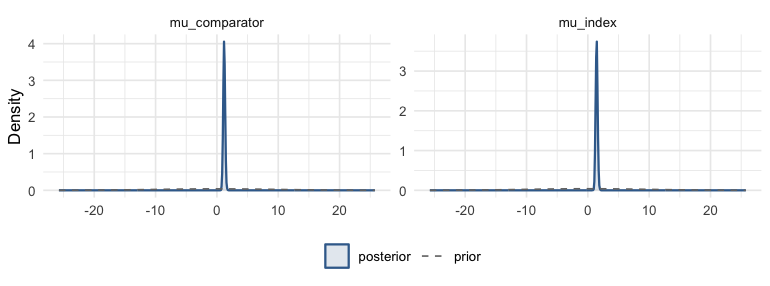
plot of chunk prior-post
Handling quasi-complete separation
With small or sparse binary data, rare events, or a covariate that
almost perfectly predicts the outcome, the maximum-likelihood logistic
fit can diverge (quasi-complete separation), and a flat or very
wide prior lets the posterior chase it to implausibly large
coefficients. A proper, substantively calibrated coefficient prior
regularizes separated directions. Gelman et al. (2008) propose a
Cauchy prior after a particular predictor scaling; a moderate Student-t
is often easier to sample, but neither family makes 2.5 universally
appropriate. No separate model is needed: the same
prior_beta argument accepts a Student-t (or Cauchy)
prior:
# Student-t coefficients (df 3-7 is a robust default), autoscaled as above:
fit_sep <- mlumr(dat, model = "spfa",
                 prior_beta = prior_student_t(df = 5, 0, 2.5, autoscale = TRUE))
# prior_cauchy(0, 2.5) is the df = 1 special case (heaviest tails).
Use prior-predictive checks to set plausible scales and
prior_sensitivity() to report how the result changes across
the scales examined.
Convergence
mlumr() warns automatically about divergences, treedepth
saturation, high \hat R, and low
effective sample size. They are clean here:
data.frame(
  n_divergent  = fit_spfa$diagnostics$n_divergent,
  max_treedepth = fit_spfa$diagnostics$n_max_treedepth,
  max_Rhat     = round(max(fit_spfa$summary$Rhat, na.rm = TRUE), 3),
  min_ESS      = round(min(fit_spfa$summary$n_eff, na.rm = TRUE))
)
#>   n_divergent max_treedepth max_Rhat min_ESS
#> 1           0             0    1.003    1836
Treatment effects
marginal_effects() reports three population-standardized
binary effect measures in each population: the log odds
ratio (LOR), the risk difference
(RD), and the risk ratio
(RR). Because ML-UMR targets both populations, you
get a population-specific effect for each.
me_spfa <- marginal_effects(fit_spfa, effect = "all")
knitr::kable(me_spfa, caption = "SPFA population-standardized effects (IXE_Q4W vs SEC_300)")| variable | effect | population | mean | sd | q2.5 | q50 | q97.5 |
|---|---|---|---|---|---|---|---|
| lor_index | LOR | Index | 0.2323910 | 0.2047769 | -0.1695227 | 0.2323505 | 0.6270024 |
| lor_comparator | LOR | Comparator | 0.2332364 | 0.2056267 | -0.1698324 | 0.2326902 | 0.6304798 |
| rd_index | RD | Index | 0.0436454 | 0.0386247 | -0.0315776 | 0.0429736 | 0.1196621 |
| rd_comparator | RD | Comparator | 0.0382168 | 0.0336965 | -0.0294068 | 0.0380543 | 0.1037666 |
| rr_index | RR | Index | 1.0618581 | 0.0557177 | 0.9589326 | 1.0591640 | 1.1778672 |
| rr_comparator | RR | Comparator | 1.0505893 | 0.0450411 | 0.9631279 | 1.0494870 | 1.1405554 |
A forest plot makes the value of adjustment visible, on the log odds ratio. ML-UMR is shown in both target populations. The index population is normally the decision-relevant one for HTA, since cost-effectiveness models are built for the population a reimbursement decision is about, which is usually the index trial’s (Chandler and Ishak 2026). STC is standardized to the comparator population; the naive contrast is not standardized to either population. Showing the comparator ML-UMR row provides the like-for-like STC comparison.
me_spfa_b <- marginal_effects(fit_spfa, effect = "lor", population = "both")
me_rel_b  <- marginal_effects(fit_relaxed, effect = "lor", population = "both")
# One row per (model, population); `pop()` pulls the requested one.
pop <- function(d, which) d[d$population == which, ]
forest_df <- data.frame(
  label = c("Naive (unstandardized)", "STC (comparator)",
            "ML-UMR SPFA (index)", "ML-UMR SPFA (comparator)",
            "ML-UMR relaxed (index)", "ML-UMR relaxed (comparator)"),
  est = c(res_naive$link_effect, res_stc$link_effect,
          pop(me_spfa_b, "Index")$mean, pop(me_spfa_b, "Comparator")$mean,
          pop(me_rel_b, "Index")$mean, pop(me_rel_b, "Comparator")$mean),
  lo  = c(res_naive$ci_lower, res_stc$ci_lower,
          pop(me_spfa_b, "Index")$q2.5, pop(me_spfa_b, "Comparator")$q2.5,
          pop(me_rel_b, "Index")$q2.5, pop(me_rel_b, "Comparator")$q2.5),
  hi  = c(res_naive$ci_upper, res_stc$ci_upper,
          pop(me_spfa_b, "Index")$q97.5, pop(me_spfa_b, "Comparator")$q97.5,
          pop(me_rel_b, "Index")$q97.5, pop(me_rel_b, "Comparator")$q97.5)
)
mlumr_forest(forest_df, ref_line = 0,
             x = "Log odds ratio",
             title = "PASI 75: ixekizumab vs secukinumab",
             subtitle = "Unadjusted vs population-adjusted, in both target populations")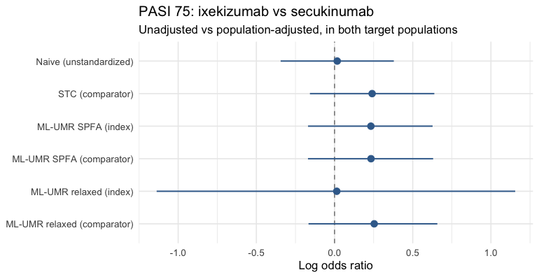
plot of chunk forest
The full set of standardized effects in both populations, as a table:
knitr::kable(marginal_effects(fit_relaxed, effect = "all", population = "both"),
caption = "Relaxed-model standardized effects, both populations")| variable | effect | population | mean | sd | q2.5 | q50 | q97.5 |
|---|---|---|---|---|---|---|---|
| lor_index | LOR | Index | 0.0141719 | 0.6172729 | -1.1375790 | 0.0264874 | 1.1553849 |
| lor_comparator | LOR | Comparator | 0.2536500 | 0.2075576 | -0.1664167 | 0.2531127 | 0.6573647 |
| rd_index | RD | Index | 0.0179156 | 0.1078882 | -0.1488600 | 0.0045542 | 0.2521100 |
| rd_comparator | RD | Comparator | 0.0414963 | 0.0339794 | -0.0270876 | 0.0415212 | 0.1080257 |
| rr_index | RR | Index | 1.0462395 | 0.1675566 | 0.8348833 | 1.0061259 | 1.4737397 |
| rr_comparator | RR | Comparator | 1.0549516 | 0.0455742 | 0.9666071 | 1.0542417 | 1.1477168 |
The population-standardized log odds ratios, in both populations,
plot straight from marginal_effects() with its
plot() method (point estimate and 95% credible interval,
faceted by measure):
plot(marginal_effects(fit_spfa, effect = "lor"))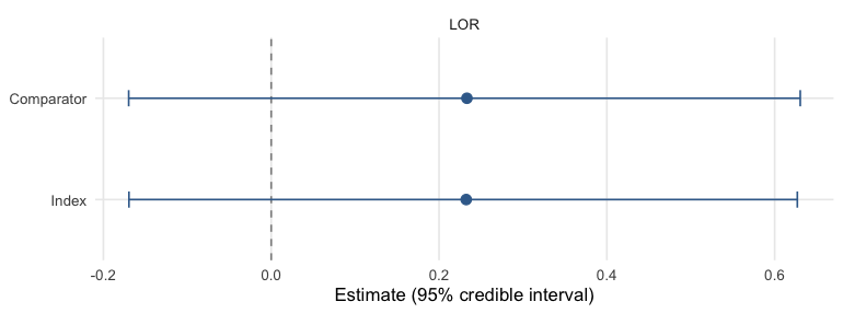
plot of chunk posterior
Absolute predictions
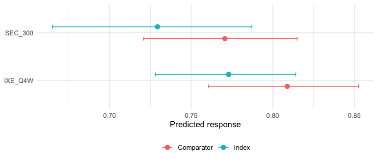
Absolute predicted response probabilities for each treatment in each
population, as a table and as a plot. plot() on a
predict() result draws the point-intervals directly, with
the two populations distinguished by color:
knitr::kable(predict(fit_spfa, population = "both", type = "response"),
caption = "Standardized PASI 75 response probabilities")| treatment | population | mean | sd | q2.5 | q50 | q97.5 |
|---|---|---|---|---|---|---|
| IXE_Q4W | Index | 0.7729681 | 0.0219597 | 0.7280789 | 0.7736964 | 0.8140666 |
| SEC_300 | Index | 0.7293227 | 0.0314229 | 0.6649613 | 0.7299364 | 0.7871844 |
| IXE_Q4W | Comparator | 0.8088424 | 0.0239865 | 0.7606818 | 0.8100515 | 0.8525781 |
| SEC_300 | Comparator | 0.7706255 | 0.0236577 | 0.7209321 | 0.7708675 | 0.8149083 |
plot of chunk predict-plot
Conditional effects
Conditional effects evaluate the contrast at specific covariate profiles rather than averaging over a population, useful for checking whether the effect is plausibly constant across the prognostic range (the SPFA assumption) or varies with the covariates:
# Weight stays in kilograms in this vignette (IPD mean about 94), unlike
# `vignette("choosing-a-method")`, which divides it by 10. Profiles must be on
# the scale the model was fitted on, or the contrast is evaluated outside the
# covariate support.
profiles <- data.frame(age = c(40, 55, 70), bsa = c(0.15, 0.30, 0.45),
                       weight = c(75, 90, 110), prevsys = c(0, 1, 1))
knitr::kable(conditional_effects(fit_spfa, newdata = profiles),
caption = "Conditional log odds ratios at three covariate profiles")| profile | effect | mean | sd | q2.5 | q50 | q97.5 |
|---|---|---|---|---|---|---|
| 1 | LINK_EFFECT | 0.2512088 | 0.2220838 | -0.1788467 | 0.2480997 | 0.6897951 |
| 1 | RD | 0.0339087 | 0.0307868 | -0.0262549 | 0.0332149 | 0.0957605 |
| 1 | RR | 1.0427288 | 0.0399764 | 0.9673283 | 1.0403847 | 1.1271305 |
| 2 | LINK_EFFECT | 0.2512088 | 0.2220838 | -0.1788467 | 0.2480997 | 0.6897951 |
| 2 | RD | 0.0514439 | 0.0457618 | -0.0357710 | 0.0502035 | 0.1429027 |
| 2 | RR | 1.0783357 | 0.0717254 | 0.9517072 | 1.0722251 | 1.2320427 |
| 3 | LINK_EFFECT | 0.2512088 | 0.2220838 | -0.1788467 | 0.2480997 | 0.6897951 |
| 3 | RD | 0.0608825 | 0.0537360 | -0.0434875 | 0.0601443 | 0.1653002 |
| 3 | RR | 1.1429823 | 0.1365554 | 0.9216199 | 1.1236565 | 1.4613458 |
Model comparison
Compare SPFA against the relaxed model with leave-one-out
cross-validation and DIC. A markedly better relaxed fit would
suggest effect modification, but the comparator coefficients
are weakly identified from a single AgD row, so treat it as suggestive
and check prior_sensitivity() (see
vignette("fitting-and-diagnostics")).
compare_models(SPFA = fit_spfa, Relaxed = fit_relaxed, criterion = "loo")
#>
#> Model Comparison (LOO)
#> ======================
#>
#>    model elpd_diff se_diff p_worse       diag_diff      diag_elpd
#>  Relaxed       0.0     0.0      NA                 1 k_psis > 0.7
#>     SPFA      -0.3     0.3    0.81 |elpd_diff| < 4 1 k_psis > 0.7
#>
#>
#> elpd_diff is the difference in expected log pointwise predictive
#> density vs the best model, and se_diff is its standard error: the
#> uncertainty about that difference, not evidence for it. Read the two
#> together. A difference small relative to se_diff is not distinguished
#> from zero by this comparison, whatever se_diff itself is.
#> Treat any ratio as a heuristic, not a decision rule, and check the
#> PSIS diagnostics and whether the difference matters for the
#> prediction you care about.
compare_models(SPFA = fit_spfa, Relaxed = fit_relaxed, criterion = "dic")
#>
#> Model Comparison (DIC)
#> ======================
#>
#>    Model    DIC   pD Delta_DIC
#>  Relaxed 368.56 6.19      0.00
#>     SPFA 368.67 6.33      0.12
#>
#> Lower DIC = better fit. Delta_DIC > 5 is a rough heuristic for
#> meaningful difference, not a formally calibrated threshold.
#> DIC should not be the sole basis for model selection.
Checking against the anchored comparison
The unanchored framing of this vignette is a construction. UNCOVER-2
and FIXTURE both randomized patients to placebo and to
etanercept, and the analysis above discards those arms.
Because they are still present in the source data, we can do something a
genuine unanchored analysis never can: check the answer against the
anchored one. multinma is a Suggests here,
used only to reach the arms mlumr does not bundle.
data("plaque_psoriasis_ipd", package = "multinma")
data("plaque_psoriasis_agd", package = "multinma")

u2 <- plaque_psoriasis_ipd[plaque_psoriasis_ipd$studyc == "UNCOVER-2", ]
u2$bsa <- u2$bsa / 100
u2$weight <- u2$weight / 10
u2$prevsys <- as.integer(u2$prevsys)
fx <- plaque_psoriasis_agd[plaque_psoriasis_agd$studyc == "FIXTURE", ]
fx$bsa_mean <- fx$bsa_mean / 100
fx$bsa_sd <- fx$bsa_sd / 100
fx$weight_mean <- fx$weight_mean / 10
fx$weight_sd <- fx$weight_sd / 10
fx$prevsys <- fx$prevsys / 100

# Conditional constancy is the assumption ML-UMR cannot test from the unanchored
# data alone. With the discarded arms it becomes testable: fit the outcome model
# in an arm both trials share, transport it to the FIXTURE population, and
# compare against what FIXTURE actually reported for that same arm.
set.seed(2026)
transport_check <- function(arm) {
  ip <- u2[u2$trtc == arm, ]
  ip <- ip[stats::complete.cases(ip[, c("pasi75", covs)]), ]
  m <- glm(pasi75 ~ age + bsa + weight + prevsys, binomial, data = ip)
  ag <- fx[fx$trtc == arm, ]
  n <- 5e4
  nd <- data.frame(age = rnorm(n, ag$age_mean, ag$age_sd),
                   bsa = rnorm(n, ag$bsa_mean, ag$bsa_sd),
                   weight = rnorm(n, ag$weight_mean, ag$weight_sd),
                   prevsys = rbinom(n, 1, ag$prevsys))
  data.frame(Arm = arm,
             `UNCOVER-2 observed` = mean(ip$pasi75),
             `Transported to FIXTURE` = mean(predict(m, nd, type = "response")),
             `FIXTURE observed` = ag$pasi75_r / ag$pasi75_n,
             check.names = FALSE)
}
knitr::kable(do.call(rbind, lapply(c("PBO", "ETN"), transport_check)), digits = 3,
caption = "Conditional-constancy check on the two arms this example discards")| Arm | UNCOVER-2 observed | Transported to FIXTURE | FIXTURE observed |
|---|---|---|---|
| PBO | 0.024 | 0.028 | 0.049 |
| ETN | 0.395 | 0.467 | 0.440 |
The etanercept row carries the information: a model fitted in UNCOVER-2’s etanercept arm predicts FIXTURE’s etanercept response to within about three percentage points of what FIXTURE reported. Conditional constancy is not exactly true, but it is close enough here that the unanchored machinery has a chance. (Placebo response is near zero in both trials and discriminates little.)
Now the anchored answers. Both trials contain etanercept, so two anchored estimates are available. The first is a Bucher indirect comparison: take each trial’s own within-trial log odds ratio against etanercept and subtract. For two studies and one common comparator that is exactly what a fixed-effect NMA returns.
lor <- function(r1, n1, r0, n0)
  c(est = log(r1 / (n1 - r1)) - log(r0 / (n0 - r0)),
    se  = sqrt(1 / r1 + 1 / (n1 - r1) + 1 / r0 + 1 / (n0 - r0)))

u2_tab <- table(u2$trtc[!is.na(u2$pasi75)], u2$pasi75[!is.na(u2$pasi75)])
lor_u2 <- lor(u2_tab["IXE_Q4W", "1"], sum(u2_tab["IXE_Q4W", ]),
              u2_tab["ETN", "1"],     sum(u2_tab["ETN", ]))
lor_fx <- lor(fx$pasi75_r[fx$trtc == "SEC_300"], fx$pasi75_n[fx$trtc == "SEC_300"],
              fx$pasi75_r[fx$trtc == "ETN"],     fx$pasi75_n[fx$trtc == "ETN"])
anchored <- unname(c(lor_u2["est"] - lor_fx["est"],
                     sqrt(lor_u2["se"]^2 + lor_fx["se"]^2)))
anchored_ci <- anchored[1] + c(-1.96, 1.96) * anchored[2]
The second is a population-adjusted ML-NMR fitted
with multinma on the same two trials, the anchored method
ML-UMR is adapted from. We fit it twice: with the covariates as
prognostic factors only, and with the full
~ (covariates) * .trt interaction that multinma’s own
plaque-psoriasis example uses. That example fits it on four studies with
treatment classes sharing their interactions; here SEC_300 is seen only
in aggregate data and shares with nothing, so its interactions are not
identified (the table’s note below says why). Both are reported so the
difference is visible rather than asserted. Note also that once
covariates interact with treatment the contrast becomes
population-specific, so multinma returns one estimate per
study; both are reported below, matching the index/comparator pair
reported for ML-UMR.
keep_u2 <- u2[u2$trtc %in% c("ETN", "IXE_Q4W"), ]
keep_u2 <- keep_u2[stats::complete.cases(keep_u2[, c("pasi75", covs)]), ]
keep_u2$prevsys <- as.numeric(keep_u2$prevsys)
keep_fx <- fx[fx$trtc %in% c("ETN", "SEC_300"), ]

net <- multinma::combine_network(
  multinma::set_ipd(keep_u2, study = studyc, trt = trtc, r = pasi75),
  multinma::set_agd_arm(keep_fx, study = studyc, trt = trtc,
                        r = pasi75_r, n = pasi75_n))
net <- multinma::add_integration(net,
  age     = multinma::distr(multinma::qgamma, mean = age_mean, sd = age_sd),
  bsa     = multinma::distr(multinma::qlogitnorm, mean = bsa_mean, sd = bsa_sd),
  weight  = multinma::distr(multinma::qgamma, mean = weight_mean, sd = weight_sd),
  prevsys = multinma::distr(multinma::qbern, prob = prevsys),
  n_int = 64)

nmr_fit <- function(form) {
  multinma::nma(net, trt_effects = "fixed", link = "logit", regression = form,
                prior_intercept = multinma::normal(0, 10),
                prior_trt = multinma::normal(0, 10),
                prior_reg = multinma::normal(0, 2.5),
                QR = TRUE, chains = 4, iter = 2000, warmup = 1000,
                seed = 2026, refresh = 0)
}

# Prognostic factors only: the anchored analogue of the SPFA model above.
fit_nmr <- nmr_fit(~ age + bsa + weight + prevsys)

# Full interaction, the formula multinma's own plaque-psoriasis example uses:
# the anchored analogue of the relaxed model. multinma fits it with treatment
# classes sharing their interactions; this sub-network has no classes, and
# SEC_300 appears only in the aggregate study.
fit_nmr_em <- nmr_fit(~ (age + bsa + weight + prevsys) * .trt)

# multinma reports SEC_300 vs IXE_Q4W; flip to match this vignette's direction.
nmr_contrast <- function(f, study = NULL) {
  d <- as.data.frame(multinma::relative_effects(f, all_contrasts = TRUE)$summary)
  d <- d[grepl("SEC_300", d$parameter) & grepl("IXE_Q4W", d$parameter), ]
  # Once covariates interact with treatment the contrast is population-specific,
  # so multinma returns one row per study: UNCOVER-2 is the index population and
  # FIXTURE the comparator, the same pair ML-UMR reports.
  if (nrow(d) > 1 && !is.null(study)) d <- d[grepl(study, d$parameter), ]
  d[1, ]
}
nmr      <- nmr_contrast(fit_nmr)
nmr_em_i <- nmr_contrast(fit_nmr_em, study = "UNCOVER-2")
nmr_em_c <- nmr_contrast(fit_nmr_em, study = "FIXTURE")

# ML-UMR is reported in both target populations so the anchored rows, which
# are comparator-population estimands, can be read against a like-for-like row.
me_spfa_i <- pop(me_spfa_b, "Index")
me_spfa_c <- pop(me_spfa_b, "Comparator")
me_rel_i  <- pop(me_rel_b, "Index")
me_rel_c  <- pop(me_rel_b, "Comparator")

knitr::kable(data.frame(
  Method = c("Naive (unadjusted)", "STC (G-computation)",
             "ML-UMR SPFA (prognostic only)",
             "ML-UMR SPFA (prognostic only)",
             "ML-UMR relaxed (effect modification)",
             "ML-UMR relaxed (effect modification)",
             "Anchored: Bucher / fixed-effect NMA",
             "Anchored: ML-NMR, prognostic only",
             "Anchored: ML-NMR, with * .trt (multinma's own model)",
             "Anchored: ML-NMR, with * .trt (multinma's own model)"),
  Anchored = c("no", "no", "no", "no", "no", "no", "yes", "yes", "yes", "yes"),
  # `naive()` contrasts the two crude outcomes; it is standardized to no
  # population, which is the point of comparing it against the adjusted rows.
  # `vignette("choosing-a-method")` uses the same label for the same reason.
  Population = c("unstandardized", "comparator", "index", "comparator",
                 "index", "comparator", "not population-specific",
                 "not population-specific", "index", "comparator"),
  LOR   = c(res_naive$link_effect, res_stc$link_effect,
            me_spfa_i$mean, me_spfa_c$mean, me_rel_i$mean, me_rel_c$mean,
            anchored[1], -nmr$mean, -nmr_em_i$mean, -nmr_em_c$mean),
  `2.5%`  = c(res_naive$ci_lower, res_stc$ci_lower,
              me_spfa_i$q2.5, me_spfa_c$q2.5, me_rel_i$q2.5, me_rel_c$q2.5,
              anchored_ci[1], -nmr[["97.5%"]],
              -nmr_em_i[["97.5%"]], -nmr_em_c[["97.5%"]]),
  `97.5%` = c(res_naive$ci_upper, res_stc$ci_upper,
              me_spfa_i$q97.5, me_spfa_c$q97.5, me_rel_i$q97.5, me_rel_c$q97.5,
              anchored_ci[2], -nmr[["2.5%"]],
              -nmr_em_i[["2.5%"]], -nmr_em_c[["2.5%"]]),
  check.names = FALSE), digits = 3,
caption = "Unanchored estimates against the anchored references, in both target populations (log odds ratio, IXE_Q4W vs SEC_300)")| Method | Anchored | Population | LOR | 2.5% | 97.5% |
|---|---|---|---|---|---|
| Naive (unadjusted) | no | unstandardized | 0.017 | -0.345 | 0.379 |
| STC (G-computation) | no | comparator | 0.240 | -0.157 | 0.638 |
| ML-UMR SPFA (prognostic only) | no | index | 0.232 | -0.170 | 0.627 |
| ML-UMR SPFA (prognostic only) | no | comparator | 0.233 | -0.170 | 0.630 |
| ML-UMR relaxed (effect modification) | no | index | 0.014 | -1.138 | 1.155 |
| ML-UMR relaxed (effect modification) | no | comparator | 0.254 | -0.166 | 0.657 |
| Anchored: Bucher / fixed-effect NMA | yes | not population-specific | 0.208 | -0.265 | 0.682 |
| Anchored: ML-NMR, prognostic only | yes | not population-specific | 0.157 | -0.366 | 0.665 |
| Anchored: ML-NMR, with * .trt (multinma’s own model) | yes | index | -8.377 | -21.582 | 0.344 |
| Anchored: ML-NMR, with * .trt (multinma’s own model) | yes | comparator | -10.521 | -25.689 | -1.552 |
The last two rows should not be interpreted substantively. The
* .trt formula is the one multinma’s own plaque-psoriasis
example uses, but that example fits it on four studies, three of them
patient-level, with the treatments grouped into classes and
class_interactions = "common", so every treatment in a
class shares one set of interactions and that set is informed by every
study in which any member of the class appears. Here both studies keep
their ETN arm, so treatment does vary within each of them; what fails is
the SEC_300 side of the network. UNCOVER-2 is patient-level data, and
the IXE_Q4W interactions are identified from it because the contrast
against ETN is observed across individuals with different covariate
values. SEC_300 appears only in FIXTURE, which is aggregate: its arm is
a single proportion, and with no class to borrow from, the SEC_300 side
of the model has five parameters of its own, a main effect and four
interaction slopes. One number cannot pin five parameters, so the
SEC_300 interactions come from the prior rather than the data, and the
IXE_Q4W versus SEC_300 contrast inherits that in both populations,
because how it moves between them is set by the difference between the
two interaction vectors. It is the evidence structure, aggregate on one
side with nothing to share, that fails to identify them, not the number
of studies. The fits converge and return estimates, but the intervals
are very wide, which is the expected signature of weak identification
rather than a usable result. Reporting both populations makes this
visible: the index and comparator values differ by more than two log
odds ratios, and that difference is set by interaction slopes the data
never informed, so it says nothing about how the contrast really varies
between the populations. A large difference is not by itself a sign of
weak identification, since strong, well-estimated effect modification
would produce one too; the width of the intervals is, and here it is the
width that rules these rows out. They are included so that both their
width and their disagreement can be compared with the rows above.
Setting those rows aside, the two identified anchored estimates agree with each other, and the SPFA model agrees with both of them in both populations. Everything that adjusts for the covariate imbalance lands in a narrow band of log odds ratios, while the naive comparison sits roughly 0.2 away from all of them. That is what population adjustment is supposed to buy, and it is only checkable because this example was built by cutting a connected network apart.
The relaxed model is the instructive exception, and it is only visible because both populations are shown. Its comparator-population estimate sits in the same narrow band as everything else, but its index-population estimate collapses back toward the naive value with an interval spanning more than two log odds ratios. Nothing about the data changed between those two rows: a single aggregate row constrains the comparator coefficients only through one combination with the comparator intercept, and the index-population estimand extrapolates them across the IPD covariate distribution. A reader shown only the comparator row would conclude the relaxed model was fine here.
One detail worth noticing: the unanchored interval is narrower than either anchored one. That is not extra information, it is the shared-prognostic-factor assumption doing work that randomization does in the anchored analyses. The interval is conditional on an assumption the anchored estimates do not need, so a tighter unanchored interval should never be read as a better answer.
Interpretation
- The naive log odds ratio mixes the treatment contrast with between-study differences, including prognostic-factor imbalance.
- In this example STC and ML-UMR SPFA both standardize over the named covariates and broadly agree. ML-UMR reports posterior uncertainty and effects in both populations, which matters when the decision population is not the comparator’s.
- The relaxed model relaxes the shared-effect assumption but pays for it in precision here, because the comparator-specific coefficients lean on one aggregate row.
Data provenance.
psoriasis_ipd/psoriasis_agdare bundled with mlumr, copied verbatim from the GPL-3multinmapackage (Phillippo 2024) (plaque_psoriasis_ipd/plaque_psoriasis_agd), which provides simulated IPD resembling the UNCOVER-2 (Griffiths et al. 2015) and FIXTURE (Langley et al. 2014) trials. This unanchored two-study framing is for illustration; the trials were not designed for a head-to-head indirect comparison.