Introduction to ML-UMR: Multilevel Unanchored Meta-Regression

Introduction

The mlumr package implements Multilevel Unanchored Meta-Regression (ML-UMR) for population-adjusted indirect comparisons in disconnected networks. This tutorial will guide you through the complete workflow from data preparation to model fitting and interpretation.

When to Use ML-UMR

ML-UMR is appropriate when:

You have individual patient data (IPD) for one treatment (the “index” treatment)
You have only aggregate data (AgD) for another treatment (the “comparator” treatment)
There is no common comparator linking the two studies (unanchored comparison)
There are population imbalances in prognostic factors between studies
You want to perform population-adjusted indirect comparisons

Key Features

Bayesian multilevel regression framework
Quasi-Monte Carlo (QMC) integration with Gaussian copula for aggregate data
Shared Prognostic Factor Assumption (SPFA) testing
Marginal effects in multiple populations
Model comparison via DIC

Installation

# Install dependencies
install.packages(c("cmdstanr", "dplyr", "tidyr", "ggplot2", "posterior",
                   "randtoolbox", "copula", "tibble", "rlang", "purrr", "glue"))

# Install CmdStan
cmdstanr::install_cmdstan()

# Install mlumr
devtools::install_local("path/to/mlumr")

library(mlumr)
library(dplyr)
library(ggplot2)

Example: Simulated Data

For this tutorial, we’ll use simulated data to demonstrate the ML-UMR workflow. In practice, you would use your own IPD and AgD.

Generate Simulation Data

Let’s generate data for an unanchored comparison with two prognostic factors:

set.seed(123)

# Scenario where SPFA holds (no effect modification)
data <- generate_simulation_data(
  n_index = 200,              # Sample size for index treatment (IPD)
  n_comparator = 150,         # Sample size for comparator treatment (AgD)
  n_covariates = 2,           # Number of prognostic factors
  effect_modification = "none", # SPFA holds
  population_shift = 0.5,     # Imbalance between populations
  correlation = 0.3,          # Correlation between covariates
  seed = 123
)

# View the data structure
print(data)
#> ML-UMR Simulation Data
#> ======================
#> 
#> Design:
#>   Likelihood: binomial 
#>   Index treatment (IPD): n = 200 
#>     Events: 82 
#>   Comparator treatment (AgD): 1 subgroups/studies
#>     Total n = 150 , Total events = 104 
#>   Number of covariates: 2 
#>   Effect modification: none 
#> 
#> True Parameters:
#>   mu_index = -0.5 
#>   mu_comparator = -0.3 
#>   beta_index: 0.5, 1 
#>   beta_comparator: 0.5, 1 
#> 
#> True Marginal Effects:
#>   LOR (index pop): -0.157 
#>   LOR (comparator pop): -0.153 
#>   RD (index pop): -0.038 
#>   RD (comparator pop): -0.037

The simulated data includes:

IPD: Individual-level data with binary outcome and covariates
AgD: Aggregate summary statistics (sample size, events, covariate means/SDs)
Truth: True parameter values (for validation)

Step 1: Set Up IPD

First, we prepare the individual patient data from the index treatment:

ipd <- set_ipd_unanchored(
  data = data$ipd,
  treatment = "treatment",
  outcome = "outcome",
  covariates = c("x1", "x2")
)

print(ipd)
#> $data
#> # A tibble: 200 × 5
#>    .study    .trt        .outcome      x1      x2
#>    <chr>     <chr>          <int>   <dbl>   <dbl>
#>  1 IPD_Study Treatment_A        1 -0.560   1.93  
#>  2 IPD_Study Treatment_A        1 -0.230   1.18  
#>  3 IPD_Study Treatment_A        1  1.56    0.215 
#>  4 IPD_Study Treatment_A        1  0.0705  0.539 
#>  5 IPD_Study Treatment_A        0  0.129  -0.356 
#>  6 IPD_Study Treatment_A        0  1.72    0.0602
#>  7 IPD_Study Treatment_A        0  0.461  -0.614 
#>  8 IPD_Study Treatment_A        0 -1.27   -0.947 
#>  9 IPD_Study Treatment_A        0 -0.687   1.37  
#> 10 IPD_Study Treatment_A        0 -0.446  -0.185 
#> # ℹ 190 more rows
#> 
#> $n
#> [1] 200
#> 
#> $n_events
#> [1] 82
#> 
#> $treatment
#> [1] "Treatment_A"
#> 
#> $covariates
#> [1] "x1" "x2"
#> 
#> $likelihood
#> [1] "binomial"
#> 
#> $type
#> [1] "ipd"
#> 
#> attr(,"class")
#> [1] "ipd_unanchored" "list"

The IPD object contains:

Standardized data structure
Sample size and event counts
Covariate names

Step 2: Set Up AgD

Next, we prepare the aggregate data from the comparator treatment:

agd <- set_agd_unanchored(
  data = data$agd,
  treatment = "treatment",
  outcome_n = "n_total",
  outcome_r = "n_events",
  cov_means = c("x1_mean", "x2_mean"),
  cov_sds = c("x1_sd", "x2_sd"),
  cov_types = c("continuous", "continuous")
)

print(agd)
#> $data
#> # A tibble: 1 × 8
#>   .study    .trt           .n    .r x1_mean x1_sd x2_mean x2_sd
#>   <chr>     <chr>       <dbl> <int>   <dbl> <dbl>   <dbl> <dbl>
#> 1 AgD_Study Treatment_B   150   104   0.418 0.966   0.626  1.04
#> 
#> $n
#> [1] 150
#> 
#> $n_events
#> [1] 104
#> 
#> $treatment
#> [1] "Treatment_B"
#> 
#> $covariates
#> [1] "x1" "x2"
#> 
#> $cov_info
#> $cov_info$x1
#> $cov_info$x1$mean_col
#> [1] "x1_mean"
#> 
#> $cov_info$x1$sd_col
#> [1] "x1_sd"
#> 
#> $cov_info$x1$type
#> [1] "continuous"
#> 
#> 
#> $cov_info$x2
#> $cov_info$x2$mean_col
#> [1] "x2_mean"
#> 
#> $cov_info$x2$sd_col
#> [1] "x2_sd"
#> 
#> $cov_info$x2$type
#> [1] "continuous"
#> 
#> 
#> 
#> $likelihood
#> [1] "binomial"
#> 
#> $type
#> [1] "agd"
#> 
#> attr(,"class")
#> [1] "agd_unanchored" "list"

For binary covariates, set cov_sds = NA and cov_types = "binary".

Step 3: Combine IPD and AgD

Combine the two data sources into a single network object:

network <- combine_unanchored(ipd, agd)
print(network)
#> Unanchored Comparison Data
#> ===========================
#> 
#> Likelihood: binomial 
#> 
#> Index treatment (IPD): Treatment_A 
#>   - N = 200 
#>   - Events = 82 (41.0%) 
#> 
#> Comparator treatment (AgD): Treatment_B 
#>   - N = 150 
#>   - Events = 104 (69.3%) 
#> 
#> Covariates ( 2 ): x1, x2 
#> 
#> Integration points: Not yet added (use add_integration_unanchored())

The package checks that:

Covariate names match between IPD and AgD
Both datasets are properly formatted

Step 4: Add Integration Points

ML-UMR uses quasi-Monte Carlo integration to handle aggregate data. We generate integration points using Sobol sequences and a Gaussian copula to preserve correlations:

network <- add_integration_unanchored(
  network,
  n_int = 64,  # Number of integration points (powers of 2 recommended)
  x1 = distr(qnorm, mean = x1_mean, sd = x1_sd),
  x2 = distr(qnorm, mean = x2_mean, sd = x2_sd)
)
#> Computing correlation matrix from IPD...
#> Added 64 integration points for AgD

print(network)
#> Unanchored Comparison Data
#> ===========================
#> 
#> Likelihood: binomial 
#> 
#> Index treatment (IPD): Treatment_A 
#>   - N = 200 
#>   - Events = 82 (41.0%) 
#> 
#> Comparator treatment (AgD): Treatment_B 
#>   - N = 150 
#>   - Events = 104 (69.3%) 
#> 
#> Covariates ( 2 ): x1, x2 
#> 
#> Integration points: 64 (QMC with Gaussian copula)

The distr() function specifies the marginal distribution for each covariate. Common distributions:

Continuous: distr(qnorm, mean = ..., sd = ...)
Binary: distr(qbern, prob = ...)
Other: Any quantile function (e.g., qgamma, qbeta)

Visualize Covariate Distributions

Compare the covariate distributions between populations:

p1 <- plot_covariate_distribution(network, "x1")
p2 <- plot_covariate_distribution(network, "x2")

print(p1)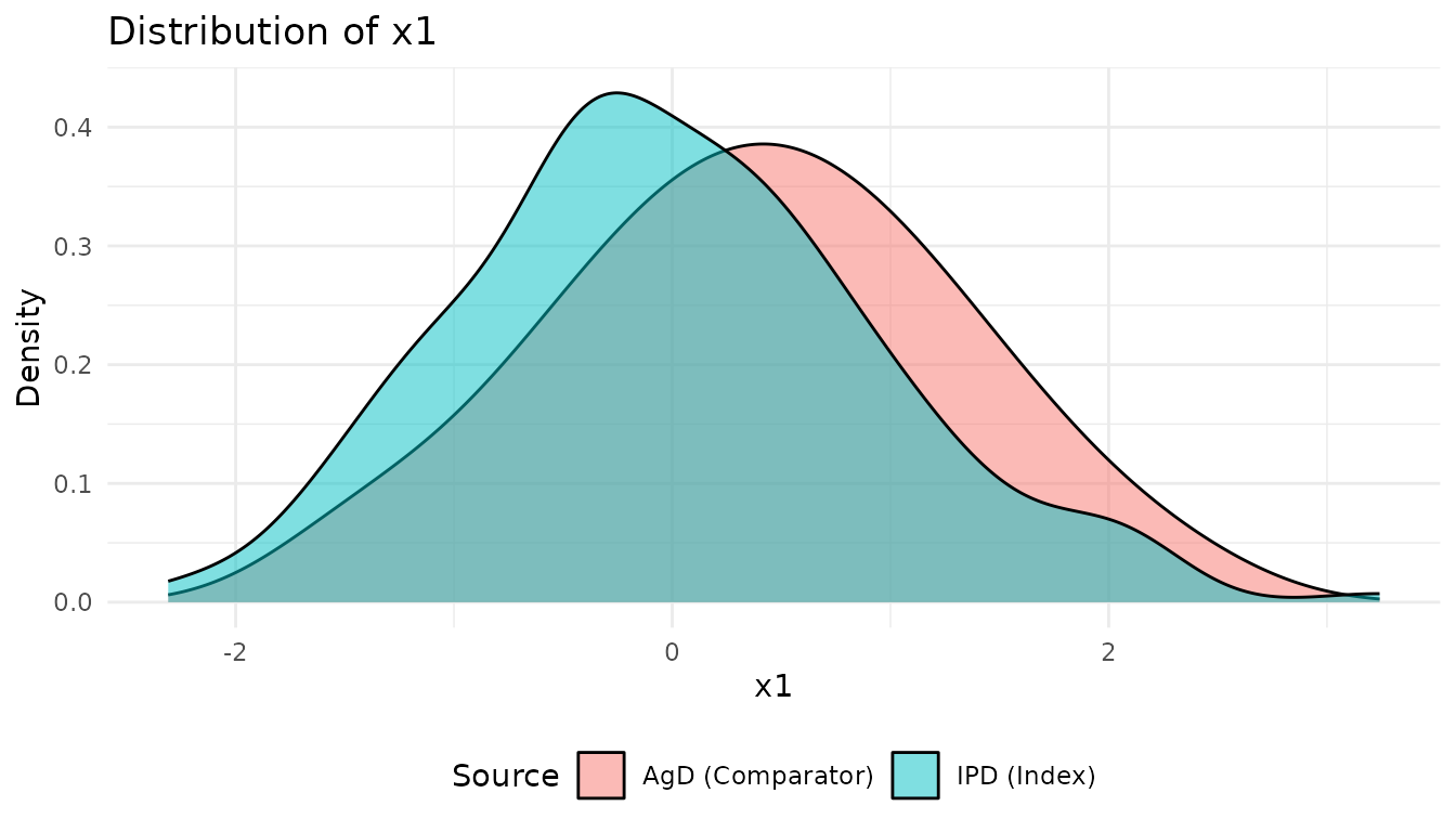

print(p2)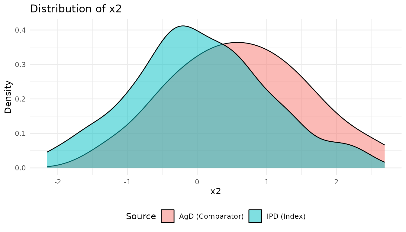

These plots show the population imbalance that ML-UMR will adjust for.

Step 5: Fit ML-UMR Model

Model with SPFA

First, fit a model that assumes the Shared Prognostic Factor Assumption (SPFA), meaning prognostic factors have the same effect on outcomes for both treatments:

fit_spfa <- mlumr(
  data = network,
  spfa = TRUE,                    # Invoke SPFA
  prior_intercept = prior_normal(0, 10),
  prior_beta = prior_normal(0, 10),
  iter_warmup = 1000,
  iter_sampling = 2000,
  chains = 4,
  seed = 123
)

print(fit_spfa)

Model with Relaxed SPFA

Now fit a model that allows treatment-specific effects (effect modification):

fit_relaxed <- mlumr(
  data = network,
  spfa = FALSE,                   # Relax SPFA
  iter_warmup = 1000,
  iter_sampling = 2000,
  chains = 4,
  seed = 123
)

print(fit_relaxed)

Step 6: Model Comparison

Compare the models using the Deviance Information Criterion (DIC):

# Calculate DIC for both models
dic_spfa <- calculate_dic(fit_spfa)
dic_relaxed <- calculate_dic(fit_relaxed)

# Compare
comparison <- compare_models(fit_spfa, fit_relaxed)

Interpretation:

Lower DIC indicates better fit
ΔDIC > 5 suggests meaningful difference
If SPFA model has lower DIC, assume shared prognostic factors
If Relaxed model has lower DIC, there is evidence of effect modification

Step 7: Extract Results

Model Summary

summary(fit_spfa)

This provides:

MCMC diagnostics (Rhat, ESS)
Intercept estimates
Regression coefficients
Marginal treatment effects

Marginal Treatment Effects

Extract marginal effects in both populations:

effects <- marginal_effects(fit_spfa, population = "both")
print(effects)

The output includes:

LOR: Log odds ratio (index vs comparator)
RD: Risk difference (index - comparator)
RR: Risk ratio (index / comparator)

In both:

Index population: Effect if comparator were given to IPD population
Comparator population: Effect if index were given to AgD population

Absolute Predictions

Get absolute probability predictions:

preds <- predict(fit_spfa, population = "both", treatment = "both")
print(preds)

Step 8: Visualizations

Marginal Effects Plot

plot(fit_spfa, type = "marginal")

Forest Plots

# Log odds ratio
plot_marginal_effects_forest(fit_spfa, effect_type = "lor")

# Risk difference
plot_marginal_effects_forest(fit_spfa, effect_type = "rd")

# Risk ratio
plot_marginal_effects_forest(fit_spfa, effect_type = "rr")

MCMC Diagnostics

# Trace plots
plot(fit_spfa, pars = c("mu_index", "mu_comparator"), type = "trace")

# Density plots
plot(fit_spfa, pars = c("mu_index", "mu_comparator"), type = "density")

Validation with Simulated Data

Since we used simulated data, we can compare estimates to true values:

truth <- data$truth

cat("True vs Estimated Log Odds Ratio (Comparator Population):\n")
cat("  True:", round(truth$lor_comparator, 3), "\n")
cat("  Estimated:", round(effects$mean[effects$variable == "lor_comparator"], 3), "\n")

Effect Modification Example

Let’s demonstrate what happens when there is strong effect modification:

# Generate data with strong effect modification
data_em <- generate_simulation_data(
  n_index = 200,
  n_comparator = 150,
  n_covariates = 2,
  effect_modification = "strong",
  seed = 456
)

# Set up and fit both models
# [Code to set up IPD, AgD, network, and integration points]

# Fit SPFA model
fit_em_spfa <- mlumr(data = network_em, spfa = TRUE, seed = 789)

# Fit Relaxed model
fit_em_relaxed <- mlumr(data = network_em, spfa = FALSE, seed = 789)

# Compare models
compare_models(fit_em_spfa, fit_em_relaxed)

# Extract effect modification parameters
delta_beta <- fit_em_relaxed$summary[grep("^delta_beta", 
                                          fit_em_relaxed$summary$variable), ]
print(delta_beta)

When effect modification is present:

Relaxed model will have lower DIC
delta_beta parameters show the difference in covariate effects between treatments
Credible intervals for delta_beta excluding zero indicate effect modification

Practical Recommendations

Sample Size

IPD: At least 100-200 patients recommended
AgD: At least 50-100 patients recommended
Larger samples provide more precise estimates

Integration Points

Use powers of 2: 32, 64, 128, 256
More points = better accuracy but slower computation
64 is usually sufficient
Test with different values to check sensitivity

Priors

Default: prior_normal(0, 10) (weakly informative)
Adjust based on prior knowledge:
- Tighter priors: prior_normal(0, 2.5)
- More vague: prior_normal(0, 20)

MCMC Settings

Warmup: 1000-2000 iterations
Sampling: 2000-4000 iterations
Chains: 4 (minimum)
Check convergence: Rhat < 1.05, ESS > 400

Model Selection

Always fit both SPFA and Relaxed models
Compare using DIC (ΔDIC > 5 is meaningful)
Check effect modification parameters in Relaxed model
Consider clinical plausibility of effect modification

Key Assumptions

ML-UMR relies on several assumptions:

No unmeasured confounding: All prognostic factors that differ between populations and modify treatment effects are measured and included
Correct functional form: Linear relationships on logit scale
Correct covariate distributions: Integration points accurately represent AgD population
SPFA (if invoked): Prognostic factors have same effect on outcomes for both treatments

SPFA is testable via model comparison, but unmeasured confounding is not. Careful consideration of what covariates to include is crucial.

Comparison with Other Methods

Method	Pros	Cons
MAIC	Simple, widely used	Strong assumptions, efficiency loss, limited to comparator population
STC	Flexible regression	Aggregation bias, limited to comparator population
ML-UMR	No aggregation bias, multiple populations, tests SPFA	Requires good knowledge of AgD distributions

Further Resources

See ?mlumr for detailed function documentation
See inst/examples/standalone_example.R for complete working example
See package vignettes for advanced topics

Session Information

sessionInfo()
#> R version 4.5.2 (2025-10-31)
#> Platform: x86_64-pc-linux-gnu
#> Running under: Ubuntu 24.04.3 LTS
#> 
#> Matrix products: default
#> BLAS:   /usr/lib/x86_64-linux-gnu/openblas-pthread/libblas.so.3 
#> LAPACK: /usr/lib/x86_64-linux-gnu/openblas-pthread/libopenblasp-r0.3.26.so;  LAPACK version 3.12.0
#> 
#> locale:
#>  [1] LC_CTYPE=C.UTF-8       LC_NUMERIC=C           LC_TIME=C.UTF-8       
#>  [4] LC_COLLATE=C.UTF-8     LC_MONETARY=C.UTF-8    LC_MESSAGES=C.UTF-8   
#>  [7] LC_PAPER=C.UTF-8       LC_NAME=C              LC_ADDRESS=C          
#> [10] LC_TELEPHONE=C         LC_MEASUREMENT=C.UTF-8 LC_IDENTIFICATION=C   
#> 
#> time zone: UTC
#> tzcode source: system (glibc)
#> 
#> attached base packages:
#> [1] stats     graphics  grDevices utils     datasets  methods   base     
#> 
#> other attached packages:
#> [1] ggplot2_4.0.2 dplyr_1.2.0   mlumr_0.1.0  
#> 
#> loaded via a namespace (and not attached):
#>  [1] sass_0.4.10         utf8_1.2.6          generics_0.1.4     
#>  [4] lattice_0.22-7      digest_0.6.39       magrittr_2.0.4     
#>  [7] evaluate_1.0.5      grid_4.5.2          RColorBrewer_1.1-3 
#> [10] mvtnorm_1.3-3       fastmap_1.2.0       jsonlite_2.0.0     
#> [13] Matrix_1.7-4        rngWELL_0.10-10     purrr_1.2.1        
#> [16] scales_1.4.0        stabledist_0.7-2    randtoolbox_2.0.5  
#> [19] numDeriv_2016.8-1.1 textshaping_1.0.4   jquerylib_0.1.4    
#> [22] cli_3.6.5           rlang_1.1.7         pspline_1.0-21     
#> [25] gsl_2.1-9           withr_3.0.2         cachem_1.1.0       
#> [28] yaml_2.3.12         tools_4.5.2         copula_1.1-6       
#> [31] vctrs_0.7.1         R6_2.6.1            stats4_4.5.2       
#> [34] lifecycle_1.0.5     ADGofTest_0.3       fs_1.6.6           
#> [37] ragg_1.5.0          pcaPP_2.0-5         pkgconfig_2.0.3    
#> [40] desc_1.4.3          pkgdown_2.2.0       pillar_1.11.1      
#> [43] bslib_0.10.0        gtable_0.3.6        glue_1.8.0         
#> [46] systemfonts_1.3.1   xfun_0.56           tibble_3.3.1       
#> [49] tidyselect_1.2.1    knitr_1.51          farver_2.1.2       
#> [52] htmltools_0.5.9     labeling_0.4.3      rmarkdown_2.30     
#> [55] compiler_4.5.2      S7_0.2.1

References

Chandler, C. & Ishak, J. (2025). “Anchors Away: Navigating Unanchored Indirect Comparisons With Multilevel Unanchored Meta-Regression (ML-UMR).” ISPOR Europe 2025.

Phillippo, D.M., et al. (2020). “Multilevel Network Meta-Regression for population-adjusted treatment comparisons.” Journal of the Royal Statistical Society: Series A, 183(3):1189-1210.

Ahmad Sofi-Mahmudi

2026-02-06